Project 2

Predicting pH in Beverage Manufacturing

library(readxl)
library(openxlsx)
library(caret)
library(dplyr)
library(tidyr)
library(tibble)
library(purrr)
library(ggplot2)
library(patchwork)
library(flextable)

# Model engines reached through caret::train()
library(pls)           # pls
library(glmnet)        # glmnet
library(earth)         # earth (MARS)
library(kernlab)       # svmRadial
library(randomForest)  # rf
library(gbm)           # gbm
library(Cubist)        # cubist
library(RANN)          # required by preProcess(method = "knnImpute")

PATH_MODEL <- "../resources/StudentData - TO MODEL.xlsx"
PATH_SCORE <- "../resources/StudentEvaluation- TO PREDICT.xlsx"
PATH_OUT   <- "../resources/PH_Predictions_Group3.xlsx"

SEED <- 624
set.seed(SEED)

proj_navy   <- "#1B3A5C"
proj_teal   <- "#2E8B8B"
proj_grey   <- "#6B7280"
proj_orange <- "#E8743B"

theme_proj <- function() {
  theme_bw(base_size = 12) +
    theme(
      plot.title    = element_text(face = "bold", color = proj_navy, size = 13),
      plot.subtitle = element_text(color = proj_grey, size = 10),
      axis.title    = element_text(color = proj_navy),
      panel.grid.minor = element_blank(),
      legend.position  = "bottom",
      legend.title     = element_blank()
    )
}

style_ft <- function(tbl, digits = 1) {
  tbl |>
    flextable() |>
    colformat_double(digits = digits) |>
    fontsize(size = 9, part = "all") |>
    align(align = "center", part = "all") |>
    autofit()
}

# Workbooks have been re-saved from Excel to fix a header encoding problem
read_raw <- function(path) as.data.frame(read_excel(path))

read_data <- function(path) {
  df <- read_raw(path)
  names(df) <- make.names(names(df))
  if (!"PH" %in% names(df)) stop("No PH column in ", path)
  if (all(is.na(df$Brand.Code))) stop("Brand.Code read as all NA in ", path)
  df
}

raw_model <- read_data(PATH_MODEL)
raw_score <- read_data(PATH_SCORE)

n_measurements <- ncol(raw_model) - 1

# Rows with no PH are dropped. Imputing the response would fabricate the target.
n_dropped_ph <- sum(is.na(raw_model$PH))
model_df     <- raw_model |> filter(!is.na(PH))

# Unknown is its own level. Unseen brands map here too, so scoring never fails.
BRAND_LEVELS <- c("A", "B", "C", "D", "Unknown")

encode_brand <- function(df) {
  b <- as.character(df$Brand.Code)
  b[is.na(b) | !(b %in% BRAND_LEVELS)] <- "Unknown"
  df$Brand.Code <- factor(b, levels = BRAND_LEVELS)
  df
}

# Flags MFR dropout, in case the outage itself is informative.
add_mfr_flag <- function(df) {
  df$MFR.Missing <- as.integer(is.na(df$MFR))
  df
}

model_df <- model_df |> encode_brand() |> add_mfr_flag()
score_df <- raw_score |> encode_brand() |> add_mfr_flag()

y_all     <- model_df$PH
X_all_raw <- model_df |> select(-PH)
X_scr_raw <- score_df |> select(-PH)

# Near-zero-variance is run on the numeric sensors only. Run after dummy
# encoding it would strip the Brand.Code.Unknown indicator, which we keep.
num_names   <- setdiff(names(X_all_raw), "Brand.Code")
dropped_nzv <- num_names[nearZeroVar(X_all_raw[num_names])]
X_all_raw   <- X_all_raw[setdiff(names(X_all_raw), dropped_nzv)]

dv    <- dummyVars(~ ., data = X_all_raw, fullRank = FALSE)
X_all <- as.data.frame(predict(dv, X_all_raw))

# The scoring file is realigned against the training columns rather than
# trusted, so an extra or absent column cannot silently shift the matrix.
align_to <- function(df_raw, ref_names, dv_obj) {
  out <- as.data.frame(predict(dv_obj, df_raw))
  for (nm in setdiff(ref_names, names(out))) out[[nm]] <- 0
  out[, ref_names, drop = FALSE]
}
X_scr <- align_to(X_scr_raw[names(X_all_raw)], names(X_all), dv)

# Stratified 80/20 split. The holdout is touched exactly once, at the end, to
# arbitrate between models that cross-validation cannot separate.
set.seed(SEED)
idx_train <- createDataPartition(y_all, p = 0.8, list = FALSE)

X_train <- X_all[idx_train, , drop = FALSE]
y_train <- y_all[idx_train]
X_test  <- X_all[-idx_train, , drop = FALSE]
y_test  <- y_all[-idx_train]

# MAPE is the metric models are tuned and selected on
mape <- function(obs, pred) mean(abs((obs - pred) / obs)) * 100

mape_summary <- function(data, lev = NULL, model = NULL) {
  c(caret::defaultSummary(data, lev, model),
    MAPE = mape(data$obs, data$pred))
}

# knnImpute is passed to train() rather than fit beforehand, so it is refit
# inside every fold. Fitting it once on the full training set would let each
# fold's held-out rows be imputed from their own neighbors.
ctrl <- trainControl(
  method          = "cv",
  number          = 10,
  savePredictions = "final",
  summaryFunction = mape_summary
)

PP <- c("knnImpute")

fit_model <- function(method, ...) {
  set.seed(SEED)
  train(X_train, y_train,
        method     = method,
        preProcess = PP,
        metric     = "MAPE",
        maximize   = FALSE,
        trControl  = ctrl,
        ...)
}

fit_lm     <- fit_model("lm")
fit_pls    <- fit_model("pls",    tuneLength = 15)
fit_enet   <- fit_model("glmnet", tuneLength = 10)
fit_mars   <- fit_model("earth",
                        tuneGrid = expand.grid(degree = 1:2,
                                               nprune = seq(5, 35, 5)))
fit_svm    <- fit_model("svmRadial", tuneLength = 8)
fit_rf     <- fit_model("rf",
                        tuneGrid = data.frame(mtry = c(8, 14, 20, 26)),
                        ntree = 500)
fit_gbm    <- fit_model("gbm",
                        tuneGrid = expand.grid(n.trees = c(500, 1000),
                                               interaction.depth = c(3, 5, 7),
                                               shrinkage = 0.05,
                                               n.minobsinnode = 10),
                        verbose = FALSE)
fit_cubist <- fit_model("cubist",
                        tuneGrid = expand.grid(committees = c(1, 10, 25, 50, 100),
                                               neighbors  = c(0, 5, 9)))

model_list <- list(
  "Linear Regression" = fit_lm,
  "PLS"               = fit_pls,
  "Elastic Net"       = fit_enet,
  "MARS"              = fit_mars,
  "SVM (radial)"      = fit_svm,
  "Random Forest"     = fit_rf,
  "GBM"               = fit_gbm,
  "Cubist"            = fit_cubist
)

family_map <- c(
  "Linear Regression" = "Linear",       "PLS"           = "Linear",
  "Elastic Net"       = "Linear",       "MARS"          = "Non-linear",
  "SVM (radial)"      = "Non-linear",   "Random Forest" = "Tree / rules",
  "GBM"               = "Tree / rules", "Cubist"        = "Tree / rules"
)

# Cross-validated performance next to holdout performance. The holdout column is
# the tiebreak when models are separated by less than fold-to-fold noise.
summarize_models <- function(models, X_te, y_te) {
  map_dfr(names(models), function(nm) {
    m    <- models[[nm]]
    best <- m$results[as.numeric(rownames(m$bestTune)), ]
    p_te <- predict(m, newdata = X_te)
    tibble(
      Model         = nm,
      Family        = unname(family_map[[nm]]),
      CV_MAPE       = best$MAPE,
      CV_RMSE       = best$RMSE,
      CV_Rsquared   = best$Rsquared,
      Test_MAPE     = mape(y_te, p_te),
      Test_RMSE     = caret::RMSE(p_te, y_te),
      Test_Rsquared = caret::R2(p_te, y_te)
    )
  }) |> arrange(CV_MAPE)
}

res_summary <- summarize_models(model_list, X_test, y_test)

cv_winner   <- res_summary$Model[1]
test_winner <- res_summary |> arrange(Test_MAPE) |> slice(1) |> pull(Model)

resamps <- resamples(model_list)

# Every model saw the same folds, so the top two are compared fold by fold.
top2   <- res_summary$Model[1:2]
paired <- resamps$values[, paste0(top2, "~MAPE")]
names(paired)     <- c("Leader", "Runner_up")
paired$Difference <- paired$Runner_up - paired$Leader

cv_margin <- mean(paired$Difference)
paired_se <- sd(paired$Difference) / sqrt(nrow(paired))

# CV ranks the models. The holdout only arbitrates between the top two, and only
# if their paired margin is smaller than its own standard error across folds.
cv_separated  <- cv_margin > paired_se

champion_name <- if (cv_winner == test_winner) {
  cv_winner
} else if (cv_separated) {
  cv_winner
} else if (test_winner %in% top2) {
  test_winner
} else {
  cv_winner
}

champion_cv  <- model_list[[champion_name]]
champion_row <- res_summary |> filter(Model == champion_name)

runner_up_name <- setdiff(top2, champion_name)[1]

# Fold-to-fold spread, quoted in prose as the yardstick for "small".
fold_spread <- diff(range(paired$Leader))

# Refit the champion without the flag, same tuning, same folds.
X_train_noflag <- X_train |> select(-MFR.Missing)
X_test_noflag  <- X_test  |> select(-MFR.Missing)

set.seed(SEED)
fit_noflag <- train(X_train_noflag, y_train,
                    method     = champion_cv$method,
                    preProcess = PP,
                    metric     = "MAPE",
                    maximize   = FALSE,
                    tuneGrid   = champion_cv$bestTune,
                    trControl  = ctrl)

ablation <- tibble(
  Variant   = c("With MFR missing flag", "Without MFR missing flag"),
  CV_MAPE   = c(champion_row$CV_MAPE,
                fit_noflag$results$MAPE[1]),
  Test_MAPE = c(champion_row$Test_MAPE,
                mape(y_test, predict(fit_noflag, newdata = X_test_noflag)))
)

# Scramble each predictor on the holdout and measure the MAPE it costs.
perm_importance <- function(model, X, y, n_rep = 5) {
  base <- mape(y, predict(model, newdata = X))
  set.seed(SEED)
  map_dfr(names(X), function(v) {
    drops <- vapply(seq_len(n_rep), function(i) {
      Xp <- X
      Xp[[v]] <- sample(Xp[[v]])
      mape(y, predict(model, newdata = Xp)) - base
    }, numeric(1))
    tibble(Variable = v, Importance = mean(drops), SD = sd(drops))
  }) |>
    mutate(Importance = pmax(Importance, 0)) |>
    arrange(desc(Importance))
}

vi <- perm_importance(champion_cv, X_test, y_test)

# Predictors grouped by what they physically measure.
var_groups <- list(
  "Formulation chemistry"       = c("Density", "Balling", "Balling.Lvl", "Alch.Rel"),
  "Machine state"               = c("Mnf.Flow"),
  "Fill and pressure setpoints" = c("Pressure.Vacuum", "Bowl.Setpoint", "Pressure.Setpoint",
                                    "Oxygen.Filler", "Air.Pressurer", "Fill.Pressure",
                                    "Filler.Level"),
  "Carbonation"                 = c("Carb.Volume", "Carb.Pressure", "Carb.Pressure1",
                                    "Carb.Temp", "Carb.Flow", "Carb.Rel", "PC.Volume",
                                    "PSC", "PSC.Fill", "PSC.CO2", "Fill.Ounces"),
  "Hydraulic pressure"          = c("Hyd.Pressure2", "Hyd.Pressure3", "Hyd.Pressure4"),
  "Brand"                       = grep("^Brand\\.Code", names(X_all), value = TRUE),
  "Instrumentation"             = c("MFR", "MFR.Missing", "Filler.Speed",
                                    "Temperature", "Usage.cont")
)

group_map <- tibble(
  Variable = unlist(var_groups, use.names = FALSE),
  Group    = rep(names(var_groups), lengths(var_groups))
)

# Every predictor must land in exactly one group.
stopifnot(setequal(group_map$Variable, names(X_all)))

vi <- vi |> left_join(group_map, by = "Variable")

# Permuting a whole group at once. Scrambling one member of a correlated cluster
# leaves its twin to carry the signal, which understates the group.
perm_group <- function(model, X, y, vars, n_rep = 5) {
  base <- mape(y, predict(model, newdata = X))
  set.seed(SEED)
  drops <- vapply(seq_len(n_rep), function(i) {
    Xp <- X
    for (v in vars) Xp[[v]] <- sample(Xp[[v]])
    mape(y, predict(model, newdata = Xp)) - base
  }, numeric(1))
  mean(drops)
}

# The champion against a tree ensemble, because importance turns out to depend
# on the model and not only on the data.
group_importance <- tibble(Group = names(var_groups)) |>
  mutate(
    Cubist        = map_dbl(var_groups, ~ perm_group(champion_cv, X_test, y_test, .x)),
    RandomForest  = map_dbl(var_groups, ~ perm_group(fit_rf,      X_test, y_test, .x))
  ) |>
  arrange(desc(Cubist))

# Top three groups, each represented by the member the champion relies on most.
PDP_GROUPS <- group_importance$Group[1:3]

pdp_vars <- vi |>
  filter(Group %in% PDP_GROUPS) |>
  group_by(Group) |>
  slice_head(n = 1) |>
  ungroup() |>
  arrange(match(Group, PDP_GROUPS)) |>
  pull(Variable)

# Walk each variable across its 2nd to 98th percentile, averaging over 300 rows.
partial_dep <- function(model, data, var, grid_n = 25, sample_n = 300) {
  set.seed(SEED)
  d    <- data[sample(nrow(data), min(sample_n, nrow(data))), , drop = FALSE]
  rng  <- quantile(data[[var]], c(0.02, 0.98), na.rm = TRUE)
  grid <- seq(rng[1], rng[2], length.out = grid_n)
  yhat <- vapply(grid, function(g) {
    d[[var]] <- g
    mean(predict(model, newdata = d))
  }, numeric(1))
  tibble(Variable = var, x = grid, yhat = yhat)
}

pdp_df   <- map_dfr(pdp_vars, ~ partial_dep(champion_cv, X_train, .x))

# Refit the champion on all usable rows at the winning tuning parameters, then
# score. The holdout has done its job and is folded back in.
set.seed(SEED)
champion_final <- train(X_all, y_all,
                        method     = champion_cv$method,
                        preProcess = PP,
                        metric     = "MAPE",
                        maximize   = FALSE,
                        tuneGrid   = champion_cv$bestTune,
                        trControl  = trainControl(method = "none"))

ph_pred <- as.numeric(predict(champion_final, newdata = X_scr))

# Fail loudly rather than ship a bad file.
stopifnot(length(ph_pred) == nrow(raw_score), !any(is.na(ph_pred)))

out    <- read_raw(PATH_SCORE)
out$PH <- round(ph_pred, 3)
write.xlsx(out, PATH_OUT)

Management Report

# Values the executive prose quotes inline
ph_mean <- mean(model_df$PH)

flow_df <- model_df |>
  filter(!is.na(Mnf.Flow)) |>
  mutate(State = if_else(Mnf.Flow < 0,
                         "Flow reading negative (near -100)",
                         "Flow reading zero or positive"))

state_means <- flow_df |>
  group_by(State) |>
  summarise(mean_ph = mean(PH), n = n(), .groups = "drop")

state_gap <- abs(diff(state_means$mean_ph))

# Unknown is excluded here. It is a real modeling level but it is not a brand,
# and the prose below is about how the four named brands differ.
brand_stats <- model_df |>
  filter(Brand.Code != "Unknown") |>
  group_by(Brand.Code) |>
  summarise(mean_ph = mean(PH), med_ph = median(PH), n = n(), .groups = "drop") |>
  arrange(desc(med_ph))

brand_hi <- brand_stats |> slice(1)
brand_lo <- brand_stats |> slice(n())

champion_mae <- caret::MAE(predict(champion_cv, newdata = X_test), y_test)

Business context

pH is a Key Performance Indicator on our beverage lines. It governs product safety, shelf life, carbonation behavior and taste, and it has to stay inside a narrow specification window. When it drifts outside that window the batch is held, reworked or destroyed, and the line loses time it cannot recover. Today pH is confirmed by laboratory measurement after a batch has already been produced, which means the plant learns about a problem only once it is too late to prevent it.

This project asks a practical question. Using only the sensor and setpoint readings the line already collects, can we predict pH accurately enough to act while a batch is still running, and can we identify which levers actually move it?

We analyzed 2,567 production runs across 32 process measurements, built and compared 8 modeling approaches spanning three families, and judged them on runs they had never seen. One run in five was held back from the start and used only at the end to confirm the choice.

What the data shows

Three findings shape everything that follows.

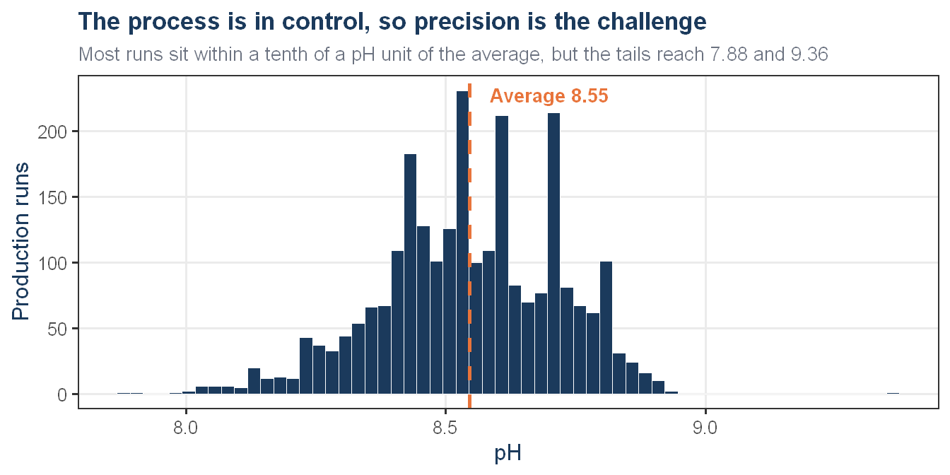
The first is that pH is already tightly controlled, which raises the bar rather than lowering it. Across the production history pH averages 8.55 with a standard deviation of only 0.173. The process is broadly in control, which is good news for the plant, and it also means that guessing the historical average every time would already be roughly right. A model only earns its keep if it can explain the small deviations. Those deviations are not hypothetical, since the record contains runs as low as 7.88 and as high as 9.36, and it is precisely those runs that get held, reworked or destroyed.

ggplot(model_df, aes(x = PH)) +
  geom_histogram(bins = 60, fill = proj_navy, color = "white", linewidth = 0.2) +
  geom_vline(xintercept = ph_mean, color = proj_orange,
             linewidth = 1, linetype = "dashed") +
  annotate("text", x = ph_mean + 0.04, y = Inf, vjust = 1.8, hjust = 0,
           label = paste0("Average ", round(ph_mean, 2)),
           color = proj_orange, fontface = "bold", size = 3.5) +
  labs(title = "The process is in control, so precision is the challenge",
       subtitle = paste0("Most runs sit within a tenth of a pH unit of the average, ",
                         "but the tails reach ", round(min(model_df$PH), 2),
                         " and ", round(max(model_df$PH), 2)),
       x = "pH", y = "Production runs") +
  theme_proj()

Exhibit 1. Distribution of pH across production runs

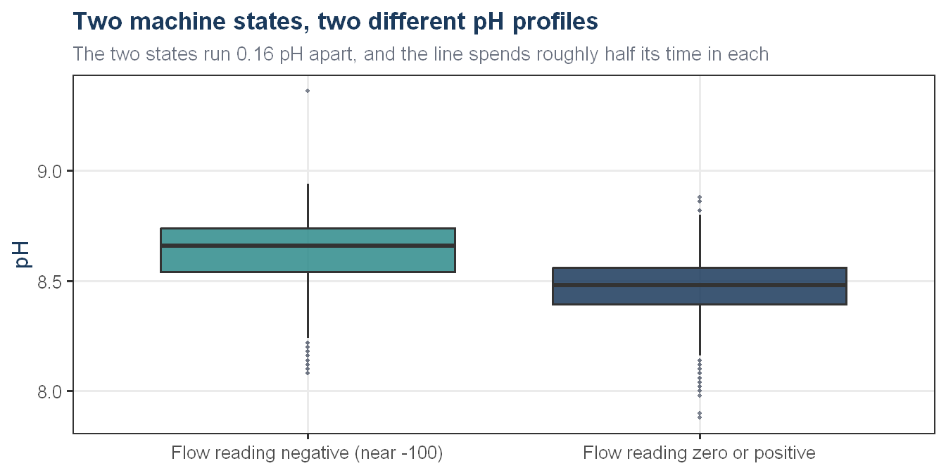
The second is that one machine reading dominates pH more than any other, and it does not behave like a sensor at all. The manufacturing flow reading, Mnf Flow, takes one of two very different states. Roughly 46 percent of runs sit at a fixed negative value near minus 100, and the rest sit at zero or spread across a positive operating range. That is the signature of an on or off condition rather than a continuously varying measurement, and the two states produce measurably different product. Runs in the negative state average a pH of 8.63, while the rest average 8.47. The 0.16 pH between them is more than twice the average error of the model we ultimately built, so this single condition moves pH further than our entire prediction uncertainty. Every model we tested found it independently.

ggplot(flow_df, aes(x = State, y = PH, fill = State)) +
  geom_boxplot(alpha = 0.85, outlier.color = proj_grey, outlier.size = 0.8) +
  scale_fill_manual(values = c(proj_teal, proj_navy)) +
  labs(title = "Two machine states, two different pH profiles",
       subtitle = sprintf("The two states run %.2f pH apart, and the line spends roughly half its time in each",
                          state_gap),
       x = NULL, y = "pH") +
  theme_proj() +
  theme(legend.position = "none")

Exhibit 2. pH separates by manufacturing flow state

The third is that brand matters, and the data is incomplete. The four brand codes run at measurably different pH levels, with Brand D highest at a median of 8.62 and Brand C lowest at 8.42, so a single plant-wide pH target is the wrong mental model. Separately, the readings themselves arrive incomplete. The flow-rate sensor MFR is absent on roughly 8 percent of historical runs and on nearly 12 percent of the runs we were asked to score, brand code is missing on about 5 percent, and most other sensors have smaller gaps. Any model that will run on the plant floor needs a defined answer for what to do when a reading does not arrive, and we return to that question below.

How we built the model

We treated this as a disciplined prediction problem and deliberately did not reach for the most complex method available. We built three families of model and let the data choose between them.

Every model was trained on the same data, prepared the same way, and judged the same way. We used ten-fold cross-validation, which means each model was trained on ninety percent of the runs and scored on the ten percent it had not seen, ten times over. Separately, one run in five was held back at the very beginning and never shown to any model during training or tuning. That holdout was opened once, at the end, to confirm the winner. This two-stage discipline is what lets us report an accuracy figure that reflects performance on genuinely new production runs rather than on runs the model has already memorized.

We also judged the models on the measure the business actually cares about. Accuracy here is reported as average percentage error, and every model was tuned and selected on that basis rather than on a statistical convenience metric.

How well the model performs

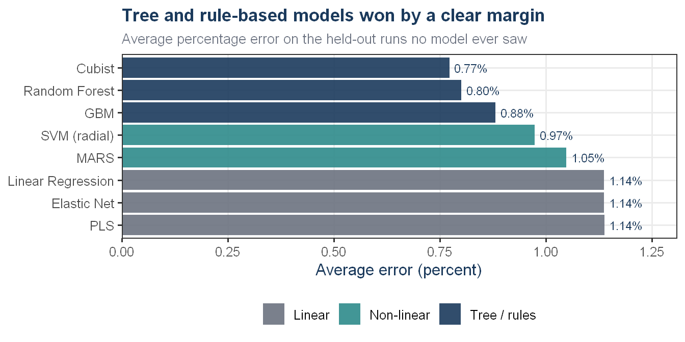
The result was not close, and it was not ambiguous. The tree and rule-based models clearly beat both the non-linear and the linear families, which is exactly what the data predicted. A straight line cannot represent an on-or-off condition, and the manufacturing flow state is precisely that.

ggplot(res_summary, aes(x = Test_MAPE, y = reorder(Model, -Test_MAPE), fill = Family)) +
  geom_col(alpha = 0.9) +
  geom_text(aes(label = sprintf("%.2f%%", Test_MAPE)),
            hjust = -0.15, size = 3, color = proj_navy) +
  scale_fill_manual(values = c("Linear"       = proj_grey,
                               "Non-linear"   = proj_teal,
                               "Tree / rules" = proj_navy)) +
  scale_x_continuous(expand = expansion(mult = c(0, 0.15))) +
  labs(title = "Tree and rule-based models won by a clear margin",
       subtitle = "Average percentage error on the held-out runs no model ever saw",
       x = "Average error (percent)", y = NULL) +
  theme_proj()

Exhibit 3. Prediction error on unseen runs, lower is better

Our champion is Cubist, a rule-based model that fits a separate local relationship inside each region of the process it identifies. It predicts pH on runs it has never seen to within an average of 0.77 percent, which in the units the plant works in is an average miss of about 0.066 pH.

That figure is worth putting next to the two things it has to beat. The gap between the two machine states is 0.16 pH, more than twice the model’s average error, so the model comfortably distinguishes conditions that genuinely move the product. And the laboratory itself reports pH in steps of 0.02, so a portion of what looks like model error is the resolution of the measurement we are being judged against.

The margin over the next best model is smaller than the margin between families, and we did not treat it as a coin flip. Cubist won the cross-validation, won the held-out confirmation, and beat the runner-up in 9 of the ten cross-validation folds. It is a consistent winner rather than a lucky one.

Exhibit 4. Champion model accuracy on unseen production runs

tibble(
  Measure = c("Average percentage error",
              "Average miss, in pH units",
              "Share of pH variation explained",
              "Production runs used to confirm this"),
  Value = c(sprintf("%.2f%%", champion_row$Test_MAPE),
            sprintf("%.3f pH", champion_mae),
            sprintf("%.0f%%", 100 * champion_row$Test_Rsquared),
            format(nrow(X_test), big.mark = ","))
) |>
  style_ft()

Measure	Value
Average percentage error	0.77%
Average miss, in pH units	0.066 pH
Share of pH variation explained	69%
Production runs used to confirm this	512

The practical test is whether the model can see a problem before the laboratory can. Its average miss of 0.066 pH is a fraction of the 0.16 pH gap between the two machine states, and it is roughly 38 percent of the standard deviation of pH across the production record. A batch drifting by a tenth of a pH unit or more would be visible to this model at the moment its readings arrive, hours before the laboratory confirms it. Whether that is early enough to act on depends on the specification window the plant holds, and we would want to calibrate the alarm threshold against that window rather than against the model.

What drives pH

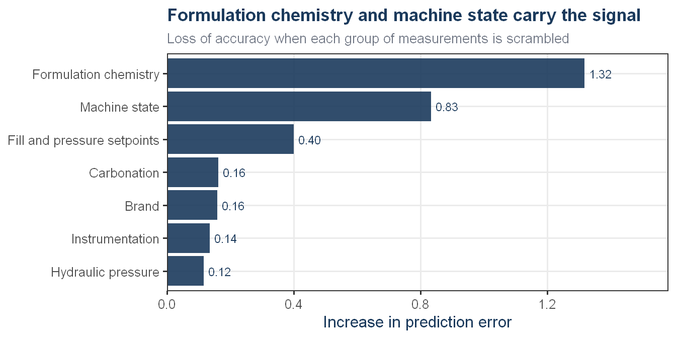
The model can be interrogated for which measurements it leans on hardest, and we did that by a deliberately conservative method. Rather than asking the model to report its own internal accounting, we scrambled each measurement in turn on runs the model had never seen and observed how much its accuracy degraded. A measurement that matters cannot be scrambled without hurting the prediction.

Because several measurements are near-duplicates of one another, we grouped them by what they physically represent and scrambled each group as a whole. Scrambling one member of a pair while its twin stays intact would understate both.

group_importance |>
  ggplot(aes(x = Cubist, y = reorder(Group, Cubist))) +
  geom_col(fill = proj_navy, alpha = 0.9) +
  geom_text(aes(label = sprintf("%.2f", Cubist)),
            hjust = -0.2, size = 3, color = proj_navy) +
  scale_x_continuous(expand = expansion(mult = c(0, 0.2))) +
  labs(title = "Formulation chemistry and machine state carry the signal",
       subtitle = "Loss of accuracy when each group of measurements is scrambled",
       x = "Increase in prediction error", y = NULL) +
  theme_proj()

Exhibit 5. What the model relies on, by measurement group

Two groups dominate. Formulation chemistry, meaning the density, balling and alcohol measurements that together describe what is actually in the tank, is the largest single influence on pH. The machine state comes second. Everything else, including the fill and pressure setpoints an operator adjusts directly, is a distant third.

There is an honest complication here that we would rather surface than bury. We repeated this exercise using a second, different model, and it reversed the top two: the chemistry group fell well below the machine state. Both models are good predictors, and both agree on which three groups matter most, but they disagree about the ordering within that top group. The reason is that the chemistry measurements are so tightly correlated with one another that different modeling approaches divide the credit among them differently. What we can say with confidence is that chemistry and machine state are the two things that matter far more than anything else, and that the exact ranking between them is a property of the model rather than a fact about the plant.

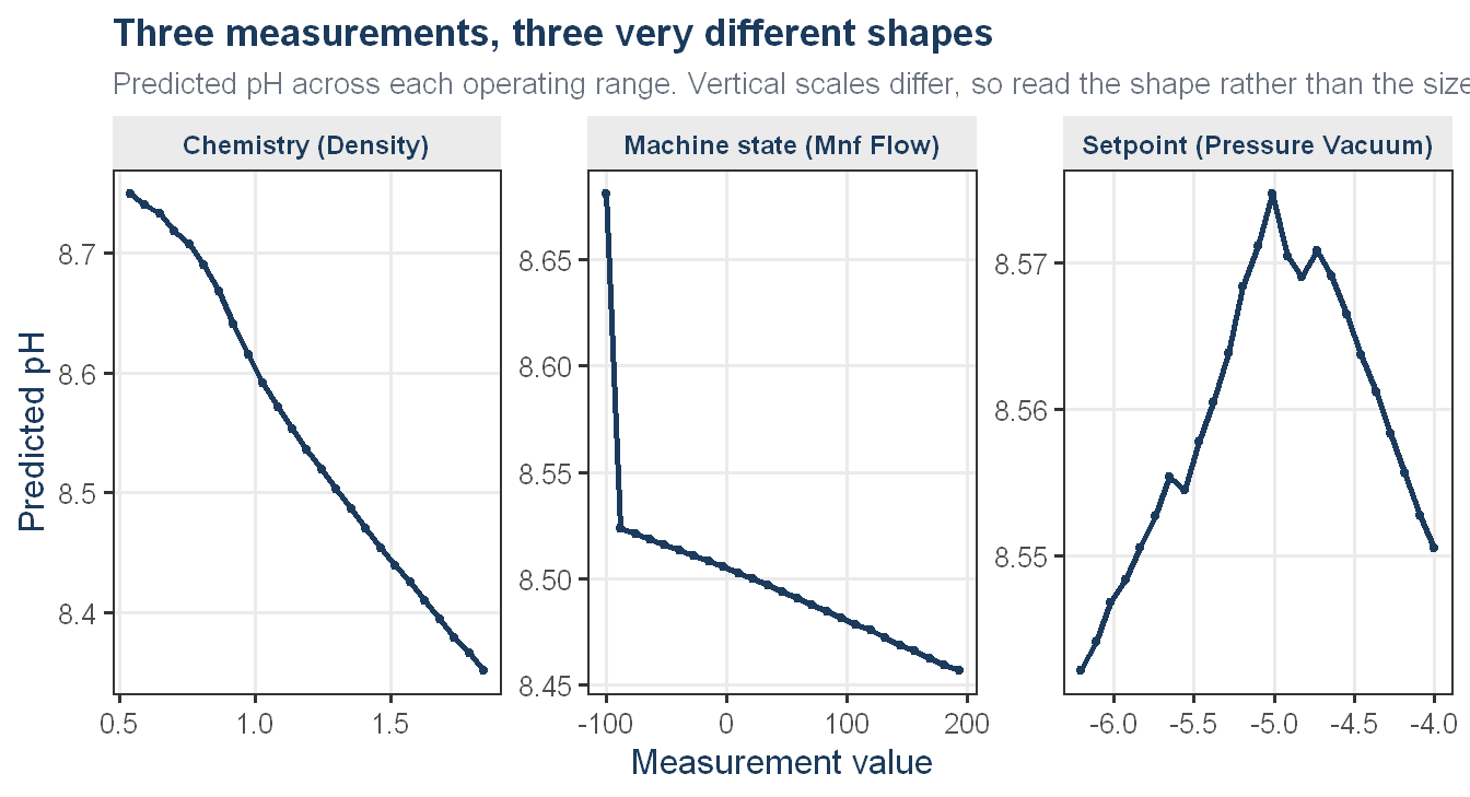
Knowing which measurements matter is only half the answer. The more useful question for an engineer is what happens to pH as each one moves. We took the champion model and walked each of the three leading measurements across its operating range while holding the rest of the process fixed, and recorded what the model predicted.

pdp_labels <- c(
  "Density"         = "Chemistry (Density)",
  "Mnf.Flow"        = "Machine state (Mnf Flow)",
  "Pressure.Vacuum" = "Setpoint (Pressure Vacuum)"
)

pdp_df |>
  mutate(Variable = factor(pdp_labels[Variable], levels = pdp_labels)) |>
  ggplot(aes(x = x, y = yhat)) +
  geom_line(color = proj_navy, linewidth = 1) +
  geom_point(color = proj_navy, size = 1) +
  facet_wrap(~ Variable, scales = "free") +
  labs(title = "Three measurements, three very different shapes",
       subtitle = "Predicted pH across each operating range. Vertical scales differ, so read the shape rather than the size",
       x = "Measurement value", y = "Predicted pH") +
  theme_proj() +
  theme(strip.background = element_rect(fill = "grey92", color = NA),
        strip.text = element_text(color = proj_navy, face = "bold", size = 9))

Exhibit 6. How predicted pH responds as the leading measurements move

The three shapes tell three different stories, and the differences are the point.

The machine state is a step, not a slope. Nearly all of its effect on pH happens in a single jump at the switch point, and once the line is running in its positive flow range, further changes in the reading barely move pH at all. This is a condition to be aware of, not a dial to be tuned. Knowing which state the line is in tells you a great deal about where pH will land. Turning the reading up or down within a state tells you almost nothing.

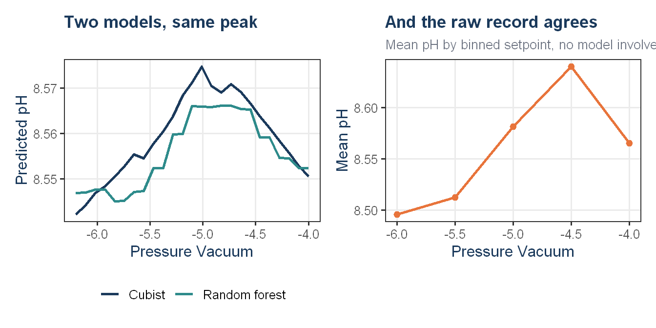
The operator setpoint has an optimum, and it is the one genuine lever we found. Pressure Vacuum is the most influential measurement on this chart that an operator can directly adjust, and predicted pH rises to a maximum in the region between roughly minus 5.1 and minus 4.5 and falls away on either side. The model’s own estimate of the effect is modest, around 0.03 pH once every other condition is held constant, and the shape is somewhat jagged because of how this particular model draws its internal boundaries. We tested it against a second, entirely different model and against the raw production record with no model involved at all, and the peak appears in the same place in all three. This is a real feature of the process rather than an artifact of our method. It is also the only place in this analysis where an operator can move pH by changing a setting rather than by changing what goes into the tank.

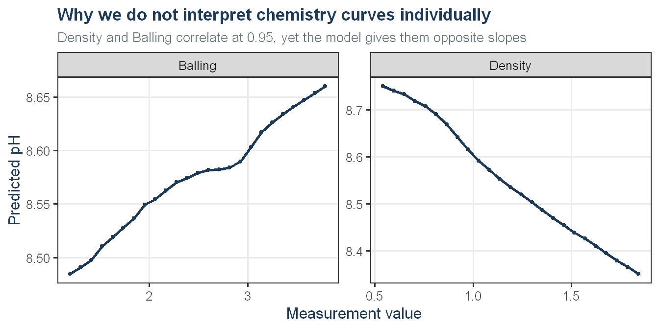
Formulation chemistry has a steep slope, and this is the one we would caution against reading literally. The chemistry measurements are near-duplicates of one another, and when we plot them individually they produce contradictory slopes, one falling while its twin rises. That contradiction is a property of the model dividing credit between two nearly identical inputs, not a property of the beverage. Chemistry unquestionably drives pH. This chart should not be used to decide which direction to move any single chemistry measurement.

What happens when the data is incomplete

Sensors fail. In the historical record the flow-rate meter MFR is missing on about 8 percent of runs, and in the 267 runs we were asked to score it is missing on nearly 12 percent. Brand code is absent on around 5 percent of historical runs. Almost every other sensor has smaller gaps. A model that refuses to produce a number whenever a reading is missing would be useless on a real production line, so we designed for incomplete data from the outset rather than treating it as a cleanup step.

When a reading is missing, we fill it in from the runs it most closely resembles. The model looks at the other readings on that same batch, finds the historical runs whose overall profile is most similar, and borrows their value for the missing measurement. This works because process variables move together. A missing flow reading can be reconstructed with reasonable confidence from filler speed, pressure and the rest of the line, because those readings carry much of the same information.

The important discipline is that the rules for filling gaps were learned only from historical production and are then fixed. They are never re-learned from the batch being scored. This matters for two reasons. It is what allows a single batch to be scored the moment it finishes, without waiting for a group of runs to compare it against. And it is what makes our accuracy figures honest, because a model that adjusted itself using the runs it was being tested on would report an accuracy it could not reproduce in the plant.

We also tested whether a missing sensor is itself a signal. It is plausible that a flow meter goes offline under particular operating conditions, in which case the absence of a reading would tell us something the reading itself would not. We built that possibility into the model as an explicit flag and measured whether it helped. It improved accuracy slightly and consistently, so we kept it, but the improvement is small. The practical conclusion is reassuring. An MFR dropout is a gap rather than a hidden warning sign, and the model handles it.

Two further cases needed a defined answer. A batch with no brand code is not guessed at. Unknown is treated as its own category, and the model learned during training how unknown-brand runs behave, so such a batch receives a real prediction rather than being forced into whichever brand happens to be most common. A brand code that has never been seen before, which will happen the first time a new product runs, is handled the same way.

The remaining case is the one to be careful about. A reading far outside anything in the historical record will still produce a number, but that number is an extrapolation, and this class of model extrapolates badly. It will quietly return a value near the edge of what it has seen before. That is exactly the situation in which a batch is most likely to be out of specification, so the deployed system should compare each incoming reading against the historical range and flag the batch for laboratory testing rather than trusting the prediction. The model is an early warning tool, not a replacement for the laboratory.

What we would change on the line

Five things follow from this analysis. Each is tied to something we measured rather than to general good practice.

1. Treat the manufacturing flow condition as a formal process state, not a sensor reading. The two states run 0.16 pH apart, and the line spends roughly half its time in each. Any pH target, control chart or alarm limit that ignores which state the line is in is averaging across two different processes. Specification limits should be set per state.

2. Run a controlled trial on the Pressure Vacuum setpoint. It is the only genuine pH lever this analysis found. Predicted pH peaks somewhere between roughly minus 5.1 and minus 4.5, and the peak appears in two independent models and in the raw production record. The effect is modest, so it is worth a deliberate trial rather than an immediate policy change, but it is the one setting on the panel that measurably moves the product.

3. Deploy the model as an in-process early warning, with a guardrail. A batch can be scored the moment its readings are available, hours before laboratory confirmation, to within an average of 0.066 pH. That is enough to flag a drifting batch while intervention is still possible. The guardrail matters as much as the model: any batch whose readings fall outside the historical range must be sent to the laboratory rather than scored, because that is precisely where the model is least reliable and where an excursion is most likely.

4. Improve the resolution of the pH measurement itself. The laboratory currently reports pH in steps of 0.02. That is a limit on quality control independent of any model, and if the specification window is narrow it may be the binding constraint on how tightly the process can be held. This is worth reviewing regardless of whether the model is deployed.

5. Do not chase individual chemistry readings. Density, balling and alcohol relation are so tightly correlated that the model cannot separate their individual effects, and neither can an engineer reading a chart. Chemistry is the largest influence on pH, but it must be managed as a formulation profile, not as a set of independent dials.

Risks and limitations

The model predicts pH. It does not explain why pH moves. Every relationship in this report is an association observed in historical production, and a measurement that predicts pH well is not necessarily a measurement that causes it. Both may be responding to something upstream that nobody recorded. This is why we recommend a controlled trial on the Pressure Vacuum setpoint rather than an immediate change to standard operating procedure.

Where measurements are near-duplicates of one another, the model divides the credit between them in ways that depend on the modeling method rather than on the plant. We saw this directly, and it is the reason we report the chemistry measurements as a group rather than ranking them. It is also the reason we deliberately show two models’ answers side by side in the appendix instead of presenting one and implying it is the truth.

The model is not reliable outside the range of conditions it has seen. Presented with a batch unlike anything in the historical record, it will return a value near the edge of its experience rather than an error, and it will do so without any signal that it is guessing. This is the model’s most dangerous failure mode because it is silent, and because it occurs exactly when a batch is most likely to be out of specification. The range check recommended above is not optional.

Finally, this model reflects the plant as it ran in the historical record. Equipment is replaced, formulations are reformulated, sensors drift and recipes change. A model trained on last year’s line will quietly become less accurate on this year’s line without announcing that it has done so. Its accuracy should be re-measured against fresh laboratory results on a regular schedule, and it should be retrained when that accuracy degrades.

Technical Appendix

Setup and libraries

The analysis runs on R with caret as the modeling interface. Every model in the comparison is reached through caret::train(), so all eight share one resampling scheme, one preprocessing recipe and one selection metric. The engines behind them are pls, glmnet, earth, kernlab, randomForest, gbm and Cubist, and RANN is required by the nearest-neighbor imputation. Tables are built with flextable and plots with ggplot2 under a shared theme.

One note on the source data. The workbook as distributed has a header encoding fault that causes some readers to return blank column names and an all-missing Brand Code. Re-saving the file from Excel corrects it. The loader below asserts on both symptoms so that the failure is loud rather than silent if it ever recurs.

library(readxl)
library(openxlsx)
library(caret)
library(dplyr)
library(tidyr)
library(tibble)
library(purrr)
library(ggplot2)
library(patchwork)
library(flextable)

# Model engines reached through caret::train()
library(pls)           # pls
library(glmnet)        # glmnet
library(earth)         # earth (MARS)
library(kernlab)       # svmRadial
library(randomForest)  # rf
library(gbm)           # gbm
library(Cubist)        # cubist
library(RANN)          # required by preProcess(method = "knnImpute")

PATH_MODEL <- "../resources/StudentData - TO MODEL.xlsx"
PATH_SCORE <- "../resources/StudentEvaluation- TO PREDICT.xlsx"
PATH_OUT   <- "../resources/PH_Predictions_Group3.xlsx"

SEED <- 624
set.seed(SEED)

proj_navy   <- "#1B3A5C"
proj_teal   <- "#2E8B8B"
proj_grey   <- "#6B7280"
proj_orange <- "#E8743B"

theme_proj <- function() {
  theme_bw(base_size = 12) +
    theme(
      plot.title    = element_text(face = "bold", color = proj_navy, size = 13),
      plot.subtitle = element_text(color = proj_grey, size = 10),
      axis.title    = element_text(color = proj_navy),
      panel.grid.minor = element_blank(),
      legend.position  = "bottom",
      legend.title     = element_blank()
    )
}

style_ft <- function(tbl, digits = 1) {
  tbl |>
    flextable() |>
    colformat_double(digits = digits) |>
    fontsize(size = 9, part = "all") |>
    align(align = "center", part = "all") |>
    autofit()
}

Data description and loading

The modeling file holds 2,571 production runs and 33 columns: 32 process measurements plus the response. One measurement, Brand Code, is categorical. The remainder are continuous sensor readings and setpoints. The evaluation file holds 267 runs with the same columns and an empty PH.

4 runs have no recorded pH. They are dropped rather than imputed, because imputing the response would mean training the model on values the model itself invented. That leaves 2,567 usable runs.

# Workbooks have been re-saved from Excel to fix a header encoding problem
read_raw <- function(path) as.data.frame(read_excel(path))

read_data <- function(path) {
  df <- read_raw(path)
  names(df) <- make.names(names(df))
  if (!"PH" %in% names(df)) stop("No PH column in ", path)
  if (all(is.na(df$Brand.Code))) stop("Brand.Code read as all NA in ", path)
  df
}

raw_model <- read_data(PATH_MODEL)
raw_score <- read_data(PATH_SCORE)

n_measurements <- ncol(raw_model) - 1

# Rows with no PH are dropped. Imputing the response would fabricate the target.
n_dropped_ph <- sum(is.na(raw_model$PH))
model_df     <- raw_model |> filter(!is.na(PH))

Exploratory data analysis

Missingness

miss_df <- bind_rows(
  tibble(Variable = names(raw_model),
         Percent  = 100 * colMeans(is.na(raw_model)),
         Set      = "Modeling"),
  tibble(Variable = names(raw_score),
         Percent  = 100 * colMeans(is.na(raw_score)),
         Set      = "Evaluation")
) |>
  filter(Variable != "PH", Percent > 0)

var_order <- miss_df |>
  group_by(Variable) |>
  summarise(m = max(Percent), .groups = "drop") |>
  arrange(m) |>
  pull(Variable)

miss_df |>
  mutate(Variable = factor(Variable, levels = var_order)) |>
  ggplot(aes(x = Percent, y = Variable, fill = Set)) +
  geom_col(position = "dodge") +
  scale_fill_manual(values = c("Modeling" = proj_navy, "Evaluation" = proj_teal)) +
  labs(title = "Missingness is shallow but present in both files",
       subtitle = "Predictors with at least one missing value",
       x = "Percent missing", y = NULL) +
  theme_proj()

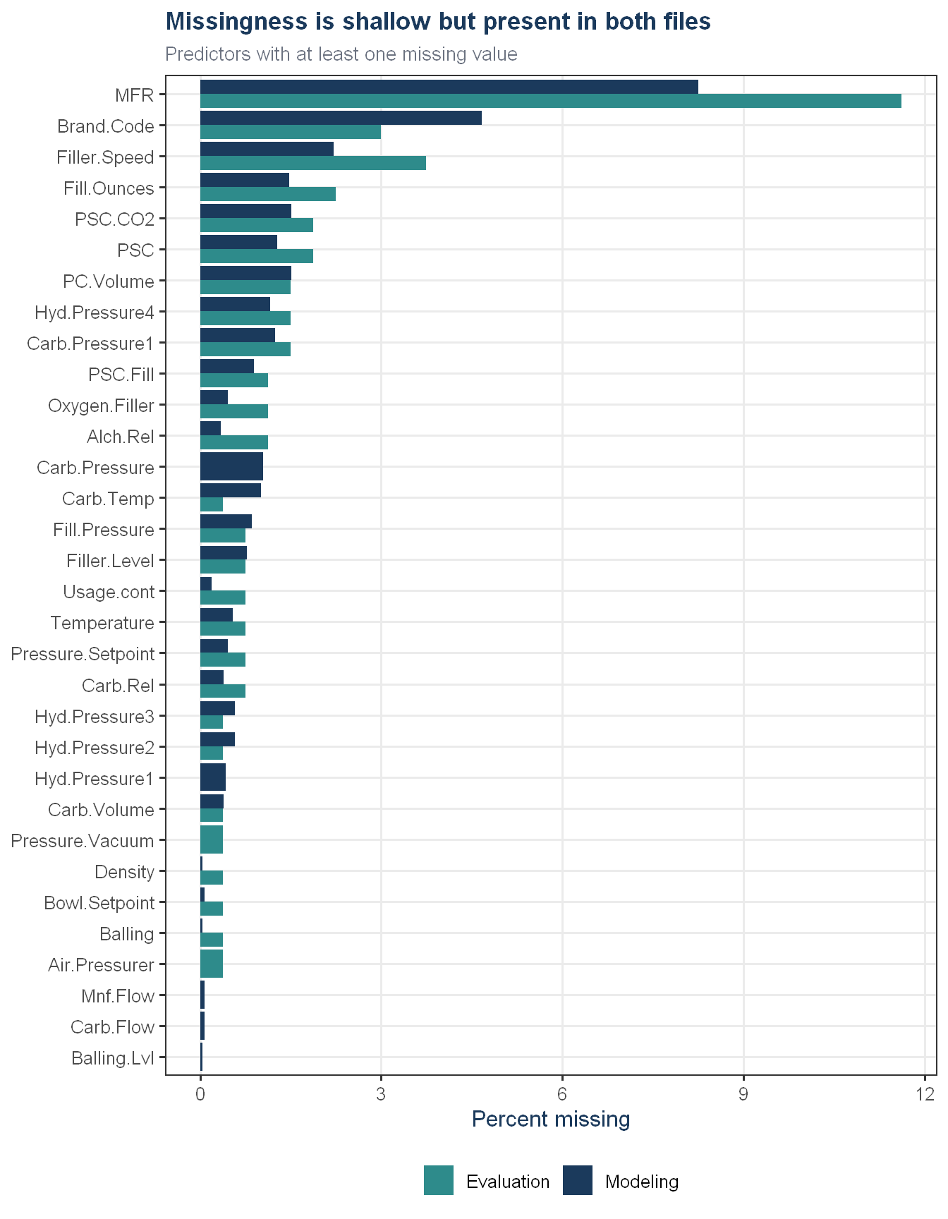
Appendix Figure A1. Percent missing by predictor, modeling against evaluation

Missingness is shallow, widespread and slightly worse in the file we have to score. MFR is the worst affected sensor by a wide margin, missing on 8.2 percent of historical runs and 11.6 percent of evaluation runs. Brand code and filler speed follow. Almost every remaining predictor has a gap somewhere, but below two percent.

The pattern that matters is the second bar in each pair. The evaluation set is not cleaner than the training set, and for several sensors it is meaningfully worse. Imputation is therefore not a data-cleaning step performed once before modeling. It is part of the production scoring path, it will run on real batches, and it has to be defined precisely enough that a single incoming run can be scored on its own, without waiting for a batch of other runs to compare it against.

The response

p_hist <- ggplot(model_df, aes(x = PH)) +
  geom_histogram(bins = 60, fill = proj_navy, color = "white", linewidth = 0.2) +
  labs(title = "Distribution of pH", x = "pH", y = "Runs") +
  theme_proj()

p_brand <- ggplot(model_df, aes(x = Brand.Code, y = PH, fill = Brand.Code)) +
  geom_boxplot(alpha = 0.85, outlier.size = 0.6, outlier.color = proj_grey) +
  scale_fill_manual(values = c(proj_navy, proj_teal, proj_grey,
                               proj_orange, "#9CA3AF")) +
  labs(title = "pH by brand", x = "Brand code", y = "pH") +
  theme_proj() +
  theme(legend.position = "none")

p_hist + p_brand

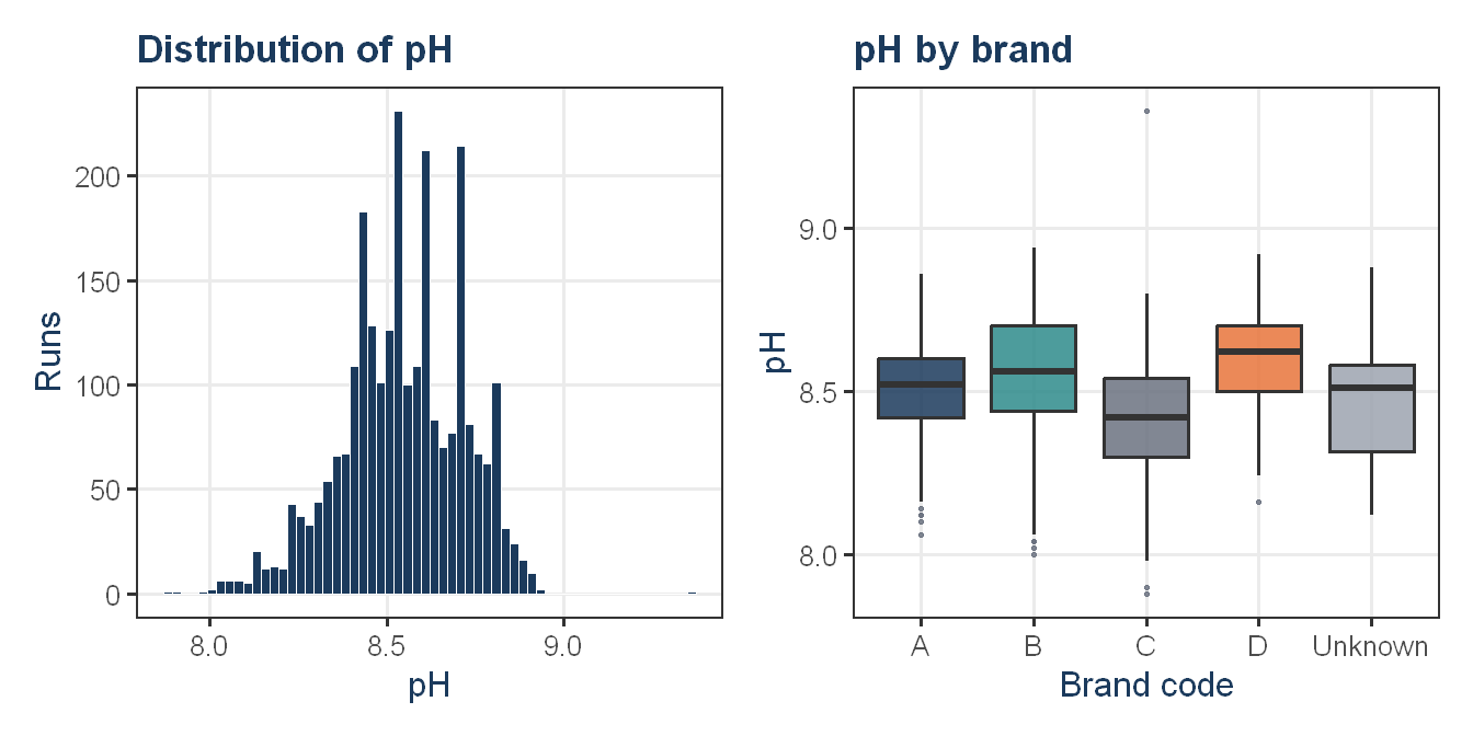
Appendix Figure A2. Response distribution and variation by brand

The response is left-skewed with a long lower tail, and the brands separate. Brand D runs highest at a median of 8.62, brand C lowest at 8.42, and the other two sit between them. That spread of 0.20 pH is roughly the same size as the 0.16 pH gap between the two machine states, so a single plant-wide pH target would be averaging across genuinely different products.

The Unknown group is the reason we did not impute brand to its most frequent value. Its distribution does not match any single observed brand. It sits near the middle with a wider spread than any of the four, which is what you would expect from a mixture of several brands rather than from one. Assigning all 120 of those runs to brand B, the most common code, would have told the model something false about every one of them. Giving Unknown its own level lets the model learn what it actually is, which is a batch whose brand we do not know.

# The response arrives on a fixed grid, which floors any model's achievable error.
ph_vals <- sort(unique(model_df$PH))
ph_step <- unique(round(diff(ph_vals), 3))

cat("Distinct pH values:", length(ph_vals), "across", nrow(model_df), "runs\n")

Distinct pH values: 52 across 2567 runs

cat("Spacing between adjacent values:", paste(sort(ph_step), collapse = ", "), "\n")

Spacing between adjacent values: 0.02, 0.08, 0.42 

cat("Champion holdout MAE:", sprintf("%.4f", champion_mae),
    "against a measurement step of", min(ph_step), "\n")

Champion holdout MAE: 0.0660 against a measurement step of 0.02 

The laboratory reports pH on a fixed grid of 0.02. Only 52 distinct values appear across 2,567 runs, and the larger gaps in the spacing above are simply values that never occurred rather than a change in resolution. This puts a floor under any model’s achievable error, since the target itself carries up to 0.01 of rounding. The floor is not binding here, because the champion’s average miss of 0.066 pH is several times larger, but it does mean a portion of what we are calling model error is measurement quantization, and it means no model can be tuned below that resolution no matter how good it gets.

Predictor structure

p_flow <- ggplot(model_df |> filter(!is.na(Mnf.Flow)), aes(x = Mnf.Flow)) +
  geom_histogram(bins = 60, fill = proj_navy, color = "white", linewidth = 0.2) +
  labs(title = "Mnf Flow is a switch, not a dial",
       subtitle = "A large mass sits at a sentinel value near -100",
       x = "Mnf Flow", y = "Runs") +
  theme_proj()

p_hyd <- model_df |>
  select(starts_with("Hyd.Pressure")) |>
  pivot_longer(everything(), names_to = "Variable", values_to = "Value") |>
  filter(!is.na(Value)) |>
  ggplot(aes(x = Value)) +
  geom_histogram(bins = 40, fill = proj_teal, color = "white", linewidth = 0.2) +
  facet_wrap(~ Variable, scales = "free", ncol = 2) +
  labs(title = "Hydraulic pressures are zero-inflated",
       x = "Reading", y = "Runs") +
  theme_proj()

p_flow + p_hyd

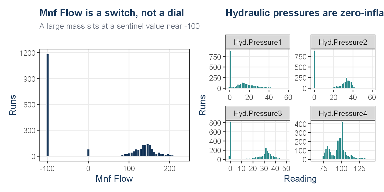
Appendix Figure A3. Machine state and zero-inflated hydraulic pressures

The left panel shows why the linear family was never going to work. 46 percent of runs sit at a single sentinel value near minus 100, a smaller group sits at exactly zero, and the remainder spread across a positive range from roughly 80 to 200. This is not a continuous measurement with a slope to estimate. It is a machine state encoded as a number. A linear model must choose one coefficient to apply across all of it, so it fits a straight line through three disconnected clusters and represents none of them. Tree and rule-based models simply split at the boundary and model each state on its own terms, which is precisely the advantage they show in Table A1.

The hydraulic pressures carry the same zero-inflated signature. Hyd.Pressure1 is the extreme case, with so much of its mass at a single value that the near-zero-variance filter removed it entirely, and it is shown here to make that decision visible rather than to hide it behind a filter.

cor_df <- X_all |>
  select(where(is.numeric)) |>
  map_dbl(~ cor(.x, y_all, use = "pairwise.complete.obs")) |>
  enframe(name = "Variable", value = "Correlation") |>
  filter(!is.na(Correlation)) |>
  arrange(desc(abs(Correlation)))

cor_df |>
  slice_head(n = 20) |>
  ggplot(aes(x = Correlation, y = reorder(Variable, Correlation),
             fill = Correlation > 0)) +
  geom_col(alpha = 0.9) +
  geom_vline(xintercept = 0, color = proj_grey) +
  scale_fill_manual(values = c("TRUE" = proj_teal, "FALSE" = proj_navy)) +
  labs(title = "No predictor has a strong linear relationship with pH",
       subtitle = "Twenty largest marginal correlations",
       x = "Correlation with pH", y = NULL) +
  theme_proj() +
  theme(legend.position = "none")

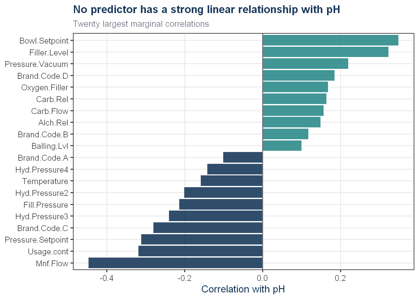
Appendix Figure A4. Marginal correlation of each predictor with pH

The strongest linear relationship anywhere in this dataset is Mnf Flow at -0.45, and nothing else exceeds 0.35 in absolute value. That result forecasts the failure of the linear family before a single model is fitted, and it explains why regularization could not rescue it. Elastic net and PLS both landed within 0.005 MAPE of ordinary least squares, because the problem was never that the linear models had too many predictors or too much collinearity. The problem is that no straight line through these predictors describes pH.

The more interesting observation is what is missing from this chart. Density and Balling, the two measurements the champion model leans on hardest, do not appear in the twenty largest marginal correlations at all. Their raw correlations with pH are 0.078 and 0.065, effectively nothing. A variable can carry almost no linear signal about pH on its own and still be the single most valuable input to a model, because its value depends on the state of the rest of the line. That gap between marginal correlation and modeled importance is the entire case for a non-linear model on this data, and it is the reason we did not screen predictors by correlation before fitting.

No correlation filter is applied. Correlated predictors do not harm tree and rule-based models, and the linear models in the comparison include a regularized variant that handles collinearity on its own terms. Removing variables before knowing which family would win would have prejudged the comparison.

Preprocessing and the missing-data strategy

The recipe is deliberately short. Brand Code is mapped to a five-level factor including Unknown and one-hot encoded. A binary indicator flags runs where MFR is missing. The near-zero-variance filter is applied to the numeric sensors, which removes 1 predictor, Hyd.Pressure1. Missing numeric values are filled by nearest-neighbor imputation, which also centers and scales as a side effect.

Two decisions in that list matter more than they look.

The near-zero-variance filter runs on the numeric sensors only, before dummy encoding rather than after. Run afterwards it would strip the Brand Code Unknown indicator, since only 4.7 percent of runs carry it, and that indicator is precisely the mechanism by which the model handles a batch with no brand.

More importantly, the imputation is fit inside the resampling loop rather than once on the full training set. This is the single most consequential line in the preprocessing code, and it is easy to get wrong. Fitting the imputation on all 2,055 training rows before splitting into folds means each fold’s held-out rows have already had their gaps filled using their own neighbors, which are sitting in the other folds. The held-out data has leaked into its own imputation, cross-validation stops being an estimate of performance on unseen data, and the reported accuracy is optimistic in a way that will not survive contact with the plant. Passing preProcess = c("knnImpute") into train() refits the imputation inside every fold on that fold’s training rows only. It costs an order of magnitude more compute and it is not optional.

The same object then imputes the evaluation runs at scoring time, using neighbors drawn from the historical record and never from the other evaluation runs. That is what allows a single batch to be scored on its own, the moment it finishes.

# Unknown is its own level. Unseen brands map here too, so scoring never fails.
BRAND_LEVELS <- c("A", "B", "C", "D", "Unknown")

encode_brand <- function(df) {
  b <- as.character(df$Brand.Code)
  b[is.na(b) | !(b %in% BRAND_LEVELS)] <- "Unknown"
  df$Brand.Code <- factor(b, levels = BRAND_LEVELS)
  df
}

# Flags MFR dropout, in case the outage itself is informative.
add_mfr_flag <- function(df) {
  df$MFR.Missing <- as.integer(is.na(df$MFR))
  df
}

model_df <- model_df |> encode_brand() |> add_mfr_flag()
score_df <- raw_score |> encode_brand() |> add_mfr_flag()

y_all     <- model_df$PH
X_all_raw <- model_df |> select(-PH)
X_scr_raw <- score_df |> select(-PH)

# Near-zero-variance is run on the numeric sensors only. Run after dummy
# encoding it would strip the Brand.Code.Unknown indicator, which we keep.
num_names   <- setdiff(names(X_all_raw), "Brand.Code")
dropped_nzv <- num_names[nearZeroVar(X_all_raw[num_names])]
X_all_raw   <- X_all_raw[setdiff(names(X_all_raw), dropped_nzv)]

dv    <- dummyVars(~ ., data = X_all_raw, fullRank = FALSE)
X_all <- as.data.frame(predict(dv, X_all_raw))

# The scoring file is realigned against the training columns rather than
# trusted, so an extra or absent column cannot silently shift the matrix.
align_to <- function(df_raw, ref_names, dv_obj) {
  out <- as.data.frame(predict(dv_obj, df_raw))
  for (nm in setdiff(ref_names, names(out))) out[[nm]] <- 0
  out[, ref_names, drop = FALSE]
}
X_scr <- align_to(X_scr_raw[names(X_all_raw)], names(X_all), dv)

The evaluation matrix is realigned against the training columns rather than trusted. A scoring file that arrives with an extra column, a missing column, or the same columns in a different order would otherwise shift the matrix silently and produce plausible-looking nonsense. Any brand code not seen in training is mapped to Unknown.

# Stratified 80/20 split. The holdout is touched exactly once, at the end, to
# arbitrate between models that cross-validation cannot separate.
set.seed(SEED)
idx_train <- createDataPartition(y_all, p = 0.8, list = FALSE)

X_train <- X_all[idx_train, , drop = FALSE]
y_train <- y_all[idx_train]
X_test  <- X_all[-idx_train, , drop = FALSE]
y_test  <- y_all[-idx_train]

The split is stratified on pH so that both partitions carry the same response distribution. The holdout is opened once, after model selection is complete.

# Sanity checks. Nothing should be left unscoreable.
cat("Predictors after encoding:", ncol(X_all), "\n")

Predictors after encoding: 36 

cat("Removed by NZV filter:", paste(dropped_nzv, collapse = ", "), "\n")

Removed by NZV filter: Hyd.Pressure1 

cat("Training rows:", nrow(X_train), "| holdout rows:", nrow(X_test),
    "| scoring rows:", nrow(X_scr), "\n")

Training rows: 2055 | holdout rows: 512 | scoring rows: 267 

cat("Scoring columns aligned to training:", identical(names(X_all), names(X_scr)), "\n")

Scoring columns aligned to training: TRUE 

cat("Scoring rows with a missing MFR reading:", sum(is.na(raw_score$MFR)), "\n")

Scoring rows with a missing MFR reading: 31 

Model specifications

Eight models across three families, one interface, one resampling scheme. Ten-fold cross-validation, tuned and selected on MAPE via a custom summary function, because MAPE is the metric the work is scored on and selecting on RMSE and reporting MAPE afterwards would be selecting on the wrong thing.

Model	Family	Why it is in the comparison
Linear regression	Linear	The baseline. If a straight line suffices, nothing more complex is justified.
PLS	Linear	Handles the heavy collinearity among the chemistry and carbonation blocks by projecting onto orthogonal components.
Elastic net	Linear	Regularized alternative that can shrink or drop correlated predictors rather than splitting coefficients between them.
MARS	Non-linear	Fits piecewise linear hinges, so it can in principle represent the Mnf Flow switch that plain linear models cannot.
SVM (radial)	Non-linear	Flexible non-parametric fit with no assumed functional form.
Random forest	Tree	Handles switches, interactions and collinearity without preprocessing. The natural favorite for this data shape.
GBM	Tree	Sequential boosting, often stronger than bagging when the signal is subtle.
Cubist	Rules	Rule-based partitions with a local linear model in each leaf, plus an optional instance-based correction. Built for exactly this kind of process data.

# MAPE is the metric models are tuned and selected on
mape <- function(obs, pred) mean(abs((obs - pred) / obs)) * 100

mape_summary <- function(data, lev = NULL, model = NULL) {
  c(caret::defaultSummary(data, lev, model),
    MAPE = mape(data$obs, data$pred))
}

# knnImpute is passed to train() rather than fit beforehand, so it is refit
# inside every fold. Fitting it once on the full training set would let each
# fold's held-out rows be imputed from their own neighbors.
ctrl <- trainControl(
  method          = "cv",
  number          = 10,
  savePredictions = "final",
  summaryFunction = mape_summary
)

PP <- c("knnImpute")

fit_model <- function(method, ...) {
  set.seed(SEED)
  train(X_train, y_train,
        method     = method,
        preProcess = PP,
        metric     = "MAPE",
        maximize   = FALSE,
        trControl  = ctrl,
        ...)
}

fit_lm     <- fit_model("lm")
fit_pls    <- fit_model("pls",    tuneLength = 15)
fit_enet   <- fit_model("glmnet", tuneLength = 10)
fit_mars   <- fit_model("earth",
                        tuneGrid = expand.grid(degree = 1:2,
                                               nprune = seq(5, 35, 5)))
fit_svm    <- fit_model("svmRadial", tuneLength = 8)
fit_rf     <- fit_model("rf",
                        tuneGrid = data.frame(mtry = c(8, 14, 20, 26)),
                        ntree = 500)
fit_gbm    <- fit_model("gbm",
                        tuneGrid = expand.grid(n.trees = c(500, 1000),
                                               interaction.depth = c(3, 5, 7),
                                               shrinkage = 0.05,
                                               n.minobsinnode = 10),
                        verbose = FALSE)
fit_cubist <- fit_model("cubist",
                        tuneGrid = expand.grid(committees = c(1, 10, 25, 50, 100),
                                               neighbors  = c(0, 5, 9)))

model_list <- list(
  "Linear Regression" = fit_lm,
  "PLS"               = fit_pls,
  "Elastic Net"       = fit_enet,
  "MARS"              = fit_mars,
  "SVM (radial)"      = fit_svm,
  "Random Forest"     = fit_rf,
  "GBM"               = fit_gbm,
  "Cubist"            = fit_cubist
)

family_map <- c(
  "Linear Regression" = "Linear",       "PLS"           = "Linear",
  "Elastic Net"       = "Linear",       "MARS"          = "Non-linear",
  "SVM (radial)"      = "Non-linear",   "Random Forest" = "Tree / rules",
  "GBM"               = "Tree / rules", "Cubist"        = "Tree / rules"
)

Model comparison and champion selection

The selection rule was fixed before the results were seen. Cross-validation ranks the models. The top two are then compared fold by fold, and if their paired margin is smaller than its own standard error across the folds, the untouched holdout arbitrates between them. If the margin clears that bar, cross-validation stands and the holdout is used only to confirm.

Appendix Table A1. Cross-validated and holdout performance, all models

res_summary |> style_ft(digits = 4)

Model	Family	CV_MAPE	CV_RMSE	CV_Rsquared	Test_MAPE	Test_RMSE	Test_Rsquared
Cubist	Tree / rules	0.7949	0.0951	0.6976	0.7729	0.0945	0.6910
Random Forest	Tree / rules	0.8228	0.0959	0.7040	0.8014	0.0966	0.6828
GBM	Tree / rules	0.9136	0.1031	0.6453	0.8812	0.1045	0.6219
SVM (radial)	Non-linear	1.0078	0.1144	0.5675	0.9740	0.1156	0.5487
MARS	Non-linear	1.0942	0.1223	0.5037	1.0485	0.1185	0.5133
Linear Regression	Linear	1.2282	0.1350	0.3936	1.1379	0.1255	0.4526
Elastic Net	Linear	1.2288	0.1350	0.3938	1.1379	0.1253	0.4550
PLS	Linear	1.2325	0.1353	0.3912	1.1381	0.1243	0.4640

resamps$values |>
  select(ends_with("~MAPE")) |>
  pivot_longer(everything(), names_to = "Model", values_to = "MAPE") |>
  mutate(Model  = sub("~MAPE$", "", Model),
         Family = family_map[Model]) |>
  ggplot(aes(x = MAPE, y = reorder(Model, -MAPE), fill = Family)) +
  geom_boxplot(alpha = 0.9, outlier.size = 0.8) +
  scale_fill_manual(values = c("Linear"       = proj_grey,
                               "Non-linear"   = proj_teal,
                               "Tree / rules" = proj_navy)) +
  labs(title = "Fold-to-fold variation is large, so the ranking must be paired",
       subtitle = "MAPE across the ten cross-validation folds",
       x = "MAPE (percent)", y = NULL) +
  theme_proj()

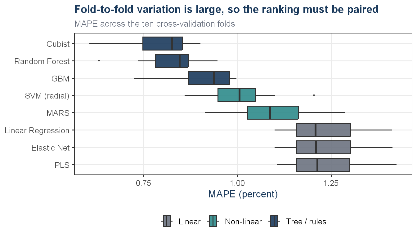
Appendix Figure A5. Cross-validation MAPE across the ten folds

The spread within any single model dwarfs the gap between models. Cubist ranges from 0.61 to 0.90 across the ten folds, a spread of 0.30, while the entire gap between it and the random forest is 0.028. Read as two independent distributions, these boxes overlap almost completely and the difference between the top two models would look like noise.

That reading would be wrong, and the reason is that the folds are not independent samples. Every model was trained and scored on the identical ten partitions, so a fold that is hard for one model is hard for all of them, and the correct comparison is paired.

The paired comparison, and the selection rule it feeds, are shown below. The rule is written so that cross-validation ranks the models and the holdout is consulted only when the paired margin between the top two is smaller than its own standard error across the folds.

# Cross-validated performance next to holdout performance. The holdout column is
# the tiebreak when models are separated by less than fold-to-fold noise.
summarize_models <- function(models, X_te, y_te) {
  map_dfr(names(models), function(nm) {
    m    <- models[[nm]]
    best <- m$results[as.numeric(rownames(m$bestTune)), ]
    p_te <- predict(m, newdata = X_te)
    tibble(
      Model         = nm,
      Family        = unname(family_map[[nm]]),
      CV_MAPE       = best$MAPE,
      CV_RMSE       = best$RMSE,
      CV_Rsquared   = best$Rsquared,
      Test_MAPE     = mape(y_te, p_te),
      Test_RMSE     = caret::RMSE(p_te, y_te),
      Test_Rsquared = caret::R2(p_te, y_te)
    )
  }) |> arrange(CV_MAPE)
}

res_summary <- summarize_models(model_list, X_test, y_test)

cv_winner   <- res_summary$Model[1]
test_winner <- res_summary |> arrange(Test_MAPE) |> slice(1) |> pull(Model)

resamps <- resamples(model_list)

# Every model saw the same folds, so the top two are compared fold by fold.
top2   <- res_summary$Model[1:2]
paired <- resamps$values[, paste0(top2, "~MAPE")]
names(paired)     <- c("Leader", "Runner_up")
paired$Difference <- paired$Runner_up - paired$Leader

cv_margin <- mean(paired$Difference)
paired_se <- sd(paired$Difference) / sqrt(nrow(paired))

# CV ranks the models. The holdout only arbitrates between the top two, and only
# if their paired margin is smaller than its own standard error across folds.
cv_separated  <- cv_margin > paired_se

champion_name <- if (cv_winner == test_winner) {
  cv_winner
} else if (cv_separated) {
  cv_winner
} else if (test_winner %in% top2) {
  test_winner
} else {
  cv_winner
}

champion_cv  <- model_list[[champion_name]]
champion_row <- res_summary |> filter(Model == champion_name)

runner_up_name <- setdiff(top2, champion_name)[1]

# Fold-to-fold spread, quoted in prose as the yardstick for "small".
fold_spread <- diff(range(paired$Leader))

cat(sprintf("%s better in %d of %d folds\n",
            top2[1], sum(paired$Difference > 0), nrow(paired)))

Cubist better in 9 of 10 folds

cat(sprintf("Mean paired margin: %.4f MAPE points\n", cv_margin))

Mean paired margin: 0.0279 MAPE points

cat(sprintf("Standard error of that margin: %.4f\n", paired_se))

Standard error of that margin: 0.0054

cat(sprintf("Worst fold for %s: %.4f\n", top2[1], min(paired$Difference)))

Worst fold for Cubist: -0.0020

cat(sprintf("CV leaders separated by more than fold noise: %s\n", cv_separated))

CV leaders separated by more than fold noise: TRUE

cat("\nCV winner:", cv_winner, "| holdout winner:", test_winner,
    "| champion:", champion_name, "\n")

CV winner: Cubist | holdout winner: Cubist | champion: Cubist 

print(champion_cv$bestTune)

   committees neighbors
14        100         5

The two routes agree, so the holdout was never asked to arbitrate. Cubist wins the cross-validation, wins the holdout, and beats the runner-up in 9 of the ten folds with a mean paired margin of 0.028 MAPE points against a standard error of 0.005. The single fold it loses, it loses by 0.002. This is a consistent winner rather than a lucky one, and it is worth being explicit that the unpaired view would not have supported that claim.

Appendix Table A2. Cubist tuning surface

champion_cv$results |>
  select(committees, neighbors, MAPE, RMSE, Rsquared, MAE) |>
  arrange(MAPE) |>
  style_ft(digits = 4) |>
  colformat_double(j = c(1, 2), digits = 0)

committees	neighbors	MAPE	RMSE	Rsquared	MAE
100	5	0.7949	0.0951	0.6976	0.0677
50	5	0.7968	0.0954	0.6958	0.0679
25	5	0.8050	0.0957	0.6942	0.0686
100	9	0.8053	0.0948	0.6996	0.0686
50	9	0.8075	0.0951	0.6976	0.0688
10	5	0.8121	0.0960	0.6924	0.0692
25	9	0.8161	0.0954	0.6958	0.0695
10	9	0.8213	0.0957	0.6941	0.0700
100	0	0.8645	0.1008	0.6675	0.0735
50	0	0.8670	0.1010	0.6655	0.0738
25	0	0.8740	0.1014	0.6621	0.0743
10	0	0.8747	0.1017	0.6586	0.0744
1	5	0.9411	0.1184	0.5644	0.0801
1	9	0.9470	0.1185	0.5592	0.0806
1	0	0.9950	0.1234	0.5198	0.0846

Two observations from the tuning surface, both worth recording.

The optimum sits at committees = 100, which is the maximum the method permits. There is no unexplored territory above it, because Cubist caps at 100 by construction. The surface is also flat above fifty, where doubling the committees buys roughly 0.002 MAPE points against a fold-to-fold spread of 0.30.

More interesting, the metrics do not agree about the instance-based correction. Five neighbors gives the best MAPE and the best MAE. Nine neighbors gives the best R-squared and, by a hair, the best RMSE. The split is not arbitrary. RMSE and R-squared are driven by squared error, so they reward the extra smoothing that nine neighbors provides, which trims the largest absolute misses. MAPE and MAE weight every run more evenly, and MAPE in particular weights each error against the size of the value being predicted, so both favor the sharper five-neighbor fit. We selected on MAPE because that is the metric this work is scored on, and the choice of metric changed the selected model. That is not a footnote. It is a reminder that the metric is a modeling decision rather than a reporting convention.

Does the MFR missingness indicator help?

MFR is the most-missing sensor in both files, and it is missing more often in the evaluation set than in the training set. If the meter tends to fail under particular operating conditions, then its absence carries information that its value does not, and a model given only an imputed value would be discarding that signal. The indicator was added to test exactly that hypothesis, and the champion was refit without it at identical tuning parameters on identical folds.

# Refit the champion without the flag, same tuning, same folds.
X_train_noflag <- X_train |> select(-MFR.Missing)
X_test_noflag  <- X_test  |> select(-MFR.Missing)

set.seed(SEED)
fit_noflag <- train(X_train_noflag, y_train,
                    method     = champion_cv$method,
                    preProcess = PP,
                    metric     = "MAPE",
                    maximize   = FALSE,
                    tuneGrid   = champion_cv$bestTune,
                    trControl  = ctrl)

ablation <- tibble(
  Variant   = c("With MFR missing flag", "Without MFR missing flag"),
  CV_MAPE   = c(champion_row$CV_MAPE,
                fit_noflag$results$MAPE[1]),
  Test_MAPE = c(champion_row$Test_MAPE,
                mape(y_test, predict(fit_noflag, newdata = X_test_noflag)))
)

Appendix Table A3. Champion with and without the MFR missingness indicator

ablation |> style_ft(digits = 4)

Variant	CV_MAPE	Test_MAPE
With MFR missing flag	0.7949	0.7729
Without MFR missing flag	0.7959	0.7748

The indicator improves accuracy on both routes, by 0.0010 MAPE points on cross-validation and 0.0019 on the holdout. The gain is small against a fold-to-fold spread of 0.30, but it points the same direction on two independent estimates, so we kept it. It also does not appear anywhere near the top of the importance rankings, which is consistent: the flag helps slightly and is not a driver.

The likely reason the gain is small is that nearest-neighbor imputation already reconstructs MFR well from the correlated instruments, principally filler speed, so the missingness carries little information that the surviving sensors do not already supply. That is a useful operational conclusion in its own right. An MFR dropout is a gap rather than a hidden signal about the state of the line.

Which measurements matter, and why the answer depends on the model

This section is the part of the analysis we would most want a reviewer to read carefully, because it produced a result we did not expect and had to test before we would report it.

Why permutation importance

Each model reports its own internal accounting of which predictors it used, but those measures are not comparable across model families and several are known to be biased. Impurity-based importance in a tree ensemble rewards predictors with many possible split points, which systematically inflates continuous sensors against binary indicators. It is also computed on the training data, so a predictor that helps the model memorize scores well even if it does not help the model predict.

Permutation importance avoids both problems. Each predictor is scrambled in turn on the holdout, the runs no model has seen, and the resulting loss of accuracy is recorded. A predictor that matters cannot be scrambled without hurting the prediction. It is model-agnostic, it is measured out of sample, and it is expressed directly in the units we care about.

# Scramble each predictor on the holdout and measure the MAPE it costs.
perm_importance <- function(model, X, y, n_rep = 5) {
  base <- mape(y, predict(model, newdata = X))
  set.seed(SEED)
  map_dfr(names(X), function(v) {
    drops <- vapply(seq_len(n_rep), function(i) {
      Xp <- X
      Xp[[v]] <- sample(Xp[[v]])
      mape(y, predict(model, newdata = Xp)) - base
    }, numeric(1))
    tibble(Variable = v, Importance = mean(drops), SD = sd(drops))
  }) |>
    mutate(Importance = pmax(Importance, 0)) |>
    arrange(desc(Importance))
}

vi <- perm_importance(champion_cv, X_test, y_test)

# Predictors grouped by what they physically measure.
var_groups <- list(
  "Formulation chemistry"       = c("Density", "Balling", "Balling.Lvl", "Alch.Rel"),
  "Machine state"               = c("Mnf.Flow"),
  "Fill and pressure setpoints" = c("Pressure.Vacuum", "Bowl.Setpoint", "Pressure.Setpoint",
                                    "Oxygen.Filler", "Air.Pressurer", "Fill.Pressure",
                                    "Filler.Level"),
  "Carbonation"                 = c("Carb.Volume", "Carb.Pressure", "Carb.Pressure1",
                                    "Carb.Temp", "Carb.Flow", "Carb.Rel", "PC.Volume",
                                    "PSC", "PSC.Fill", "PSC.CO2", "Fill.Ounces"),
  "Hydraulic pressure"          = c("Hyd.Pressure2", "Hyd.Pressure3", "Hyd.Pressure4"),
  "Brand"                       = grep("^Brand\\.Code", names(X_all), value = TRUE),
  "Instrumentation"             = c("MFR", "MFR.Missing", "Filler.Speed",
                                    "Temperature", "Usage.cont")
)

group_map <- tibble(
  Variable = unlist(var_groups, use.names = FALSE),
  Group    = rep(names(var_groups), lengths(var_groups))
)

# Every predictor must land in exactly one group.
stopifnot(setequal(group_map$Variable, names(X_all)))

vi <- vi |> left_join(group_map, by = "Variable")

# Permuting a whole group at once. Scrambling one member of a correlated cluster
# leaves its twin to carry the signal, which understates the group.
perm_group <- function(model, X, y, vars, n_rep = 5) {
  base <- mape(y, predict(model, newdata = X))
  set.seed(SEED)
  drops <- vapply(seq_len(n_rep), function(i) {
    Xp <- X
    for (v in vars) Xp[[v]] <- sample(Xp[[v]])
    mape(y, predict(model, newdata = Xp)) - base
  }, numeric(1))
  mean(drops)
}

# The champion against a tree ensemble, because importance turns out to depend
# on the model and not only on the data.
group_importance <- tibble(Group = names(var_groups)) |>
  mutate(
    Cubist        = map_dbl(var_groups, ~ perm_group(champion_cv, X_test, y_test, .x)),
    RandomForest  = map_dbl(var_groups, ~ perm_group(fit_rf,      X_test, y_test, .x))
  ) |>
  arrange(desc(Cubist))

The result, and the problem with it

Appendix Table A4. Individual permutation importance, champion model, top fifteen

vi |>
  slice_head(n = 15) |>
  select(Variable, Group, Importance, SD) |>
  style_ft(digits = 4)

Variable	Group	Importance	SD
Density	Formulation chemistry	1.1883	0.0434
Balling	Formulation chemistry	0.8439	0.0688
Mnf.Flow	Machine state	0.8020	0.0408
Alch.Rel	Formulation chemistry	0.3769	0.0345
Pressure.Vacuum	Fill and pressure setpoints	0.1554	0.0086
Balling.Lvl	Formulation chemistry	0.1228	0.0249
Brand.Code.C	Brand	0.1175	0.0184
Bowl.Setpoint	Fill and pressure setpoints	0.1059	0.0089
Oxygen.Filler	Fill and pressure setpoints	0.1049	0.0217
Usage.cont	Instrumentation	0.0697	0.0146
Air.Pressurer	Fill and pressure setpoints	0.0664	0.0091
Carb.Flow	Carbonation	0.0630	0.0122
Carb.Rel	Carbonation	0.0574	0.0066
Hyd.Pressure3	Hydraulic pressure	0.0539	0.0090
Hyd.Pressure2	Hydraulic pressure	0.0437	0.0052

Under the champion, the chemistry block occupies the top of the ranking, and Mnf Flow, which the raw correlations and every other model in this comparison identify as the dominant predictor, falls to third.

That result contradicted our expectations, so we tested whether it was an artifact of the importance measure or a property of the model. The test is a two-by-two: impurity importance and permutation importance, each applied to Cubist and to the random forest.

Appendix Table A5. Impurity against permutation, random forest, top ten

imp_rf <- varImp(fit_rf, scale = TRUE)$importance
imp_rf <- tibble(Variable = rownames(imp_rf), Impurity = imp_rf[, 1]) |>
  arrange(desc(Impurity)) |>
  slice_head(n = 10)

vi_rf <- perm_importance(fit_rf, X_test, y_test) |>
  slice_head(n = 10) |>
  select(Variable, Permutation = Importance)

bind_cols(
  imp_rf |> rename(`By impurity` = Variable, Score = Impurity),
  vi_rf  |> rename(`By permutation` = Variable, Loss = Permutation)
) |>
  style_ft(digits = 3)

By impurity	Score	By permutation	Loss
Mnf.Flow	100.000	Mnf.Flow	0.593
Brand.Code.C	33.962	Alch.Rel	0.140
Usage.cont	30.422	Brand.Code.C	0.129
Oxygen.Filler	23.739	Usage.cont	0.123
Alch.Rel	21.900	Pressure.Vacuum	0.092
Pressure.Vacuum	20.333	Oxygen.Filler	0.090
Temperature	18.599	Bowl.Setpoint	0.078
Air.Pressurer	18.514	Air.Pressurer	0.063
Balling.Lvl	17.132	Carb.Rel	0.063
Carb.Rel	15.084	Balling.Lvl	0.059

Both measures on the random forest put Mnf Flow first, and by a wide margin: impurity scores it at 100 against 34 for the next predictor, and permutation scores it at 0.593 against 0.140. They also broadly agree with each other on the rest of the ordering. So the reversal we saw under the champion is not caused by the choice of importance measure. Impurity and permutation tell the same story when applied to the same model.

The reversal is caused by the model. Note also what is absent from both random forest columns: Density and Balling, the two predictors the champion ranks first and second, do not appear in the random forest’s top ten under either measure.

Appendix Table A6. Grouped permutation importance, two models compared

group_importance |> style_ft(digits = 4)

Group	Cubist	RandomForest
Formulation chemistry	1.3171	0.2214
Machine state	0.8328	0.6258
Fill and pressure setpoints	0.3998	0.3309
Carbonation	0.1620	0.1272
Brand	0.1595	0.1681
Instrumentation	0.1352	0.1890
Hydraulic pressure	0.1167	0.0648

The grouped comparison makes the disagreement unambiguous. The two models agree on which three groups matter and agree closely on the ordering of the bottom four. They disagree, sharply, on the top two. Under Cubist, chemistry is worth 1.32 MAPE points against the machine state’s 0.83. Under the random forest, the ordering reverses.

Why the two models disagree

The chemistry measurements are near-duplicates of one another.

chem <- var_groups[["Formulation chemistry"]]
cat("Correlations among the chemistry measurements:\n")

Correlations among the chemistry measurements:

print(round(cor(X_all[chem], use = "pairwise.complete.obs"), 3))

            Density Balling Balling.Lvl Alch.Rel
Density       1.000   0.955       0.949    0.903
Balling       0.955   1.000       0.979    0.925
Balling.Lvl   0.949   0.979       1.000    0.927
Alch.Rel      0.903   0.925       0.927    1.000

cat("\nMarginal correlation of each with pH:\n")

Marginal correlation of each with pH:

print(round(cor(X_all[chem], y_all, use = "pairwise.complete.obs"), 3))

             [,1]
Density     0.078
Balling     0.065
Balling.Lvl 0.100
Alch.Rel    0.149

Every pairing correlates above 0.90, and all four have the same weak positive marginal relationship with pH. Cubist fits a local linear model inside each rule, and collinear predictors in a linear fit receive large coefficients of opposing sign that cancel one another out. Scrambling one of them alone breaks the cancellation and the surviving coefficient runs unopposed, so the error rises steeply. The random forest can only use these predictors through splits, has no coefficients to cancel, and so is unaffected.

That explanation predicts that the chemistry variables should be redundant, and that pruning to one of them should cost little. We tested that too, and the prediction was wrong.

# If the chemistry block were merely redundant, dropping three of the four
# should be nearly free.
keep_one <- setdiff(names(X_train), c("Balling", "Balling.Lvl", "Alch.Rel"))
set.seed(SEED)
fit_chem1 <- train(X_train[keep_one], y_train,
                   method = champion_cv$method, preProcess = PP,
                   metric = "MAPE", maximize = FALSE,
                   tuneGrid = champion_cv$bestTune, trControl = ctrl)

mape_all_chem <- mape(y_test, predict(champion_cv, newdata = X_test))
mape_one_chem <- mape(y_test, predict(fit_chem1,   newdata = X_test[keep_one]))

cat(sprintf("All four chemistry measurements, holdout MAPE: %.4f\n", mape_all_chem))

All four chemistry measurements, holdout MAPE: 0.7729

cat(sprintf("Density only, holdout MAPE:                    %.4f\n", mape_one_chem))

Density only, holdout MAPE:                    0.8142

Pruning to a single chemistry measurement costs 0.0413 MAPE points on the holdout, which is larger than the entire margin between the champion and the runner-up model. So the collinear-coefficient explanation is at best incomplete. If these four measurements were merely redundant restatements of one another, three of them could be discarded at little cost. They cannot. The differences between them carry real predictive information, and the champion is using it.

The disciplined position is therefore narrower than either extreme. Chemistry and machine state are the two things that matter, and both matter far more than anything else. That much survives every framing we tried. The ranking between them does not: it depends on the model, and we report both models rather than presenting one and implying it is the truth. Within the chemistry cluster we make no attribution at all, because the measurements are neither separable nor discardable, and any ranking among them would be an artifact of the method rather than a fact about the beverage.

Partial dependence

Partial dependence curves are computed on the raw predictor scale. Because imputation and scaling are held inside the model object rather than applied to the data beforehand, the matrices we hold are on the original sensor scale, and the horizontal axis is a value an engineer can act on rather than a standardized score.

The representative variable for each group is chosen as the member the champion leans on hardest, and the three groups are the three the grouped permutation results rank highest. Neither choice is hardcoded.

# Top three groups, each represented by the member the champion relies on most.
PDP_GROUPS <- group_importance$Group[1:3]

pdp_vars <- vi |>
  filter(Group %in% PDP_GROUPS) |>
  group_by(Group) |>
  slice_head(n = 1) |>
  ungroup() |>
  arrange(match(Group, PDP_GROUPS)) |>
  pull(Variable)

# Walk each variable across its 2nd to 98th percentile, averaging over 300 rows.
partial_dep <- function(model, data, var, grid_n = 25, sample_n = 300) {
  set.seed(SEED)
  d    <- data[sample(nrow(data), min(sample_n, nrow(data))), , drop = FALSE]
  rng  <- quantile(data[[var]], c(0.02, 0.98), na.rm = TRUE)
  grid <- seq(rng[1], rng[2], length.out = grid_n)
  yhat <- vapply(grid, function(g) {
    d[[var]] <- g
    mean(predict(model, newdata = d))
  }, numeric(1))
  tibble(Variable = var, x = grid, yhat = yhat)
}

pdp_df   <- map_dfr(pdp_vars, ~ partial_dep(champion_cv, X_train, .x))

chem_pdp <- map_dfr(c("Density", "Balling"), ~ partial_dep(champion_cv, X_train, .x))
chem_cor <- cor(X_all$Density, X_all$Balling, use = "pairwise.complete.obs")

# Net movement in predicted pH from one end of each curve to the other.
chem_slope <- function(v) {
  y <- chem_pdp$yhat[chem_pdp$Variable == v]
  y[length(y)] - y[1]
}

chem_pdp |>
  ggplot(aes(x = x, y = yhat)) +
  geom_line(color = proj_navy, linewidth = 1) +
  geom_point(color = proj_navy, size = 1) +
  facet_wrap(~ Variable, scales = "free") +
  labs(title = "Why we do not interpret chemistry curves individually",
       subtitle = sprintf(paste("Density and Balling correlate at %.2f,",
                                "yet the model gives them opposite slopes"),
                          chem_cor),
       x = "Measurement value", y = "Predicted pH") +
  theme_proj()

Appendix Figure A6. Two near-identical measurements, opposite modeled slopes

This figure is the evidence for that refusal rather than an assertion of it. Density and Balling correlate at 0.95, and both have the same weak positive relationship with pH in the raw data. Yet the champion gives them opposite slopes: predicted pH falls by 0.40 across the range of Density and rises by 0.18 across the range of Balling. There is no physical reading of that. Two near-identical measurements of the same underlying property cannot move pH in opposite directions. What we are seeing is a model dividing credit between two nearly interchangeable inputs, with coefficients that offset one another and only make sense in combination. Neither curve may be read as a control response, and neither should be shown to an engineer as one.

pv_raw <- model_df |>
  filter(!is.na(Pressure.Vacuum)) |>
  mutate(bin = round(Pressure.Vacuum * 2) / 2) |>
  group_by(bin) |>
  summarise(mean_ph = mean(PH), n = n(), .groups = "drop") |>
  filter(n >= 30)

pv_models <- bind_rows(
  partial_dep(champion_cv, X_train, "Pressure.Vacuum") |> mutate(Source = "Cubist"),
  partial_dep(fit_rf,      X_train, "Pressure.Vacuum") |> mutate(Source = "Random forest")
)

pv_peak <- function(src) {
  d <- pv_models |> filter(Source == src)
  d$x[which.max(d$yhat)]
}

p_pv_model <- ggplot(pv_models, aes(x = x, y = yhat, color = Source)) +
  geom_line(linewidth = 1) +
  scale_color_manual(values = c("Cubist" = proj_navy, "Random forest" = proj_teal)) +
  labs(title = "Two models, same peak", x = "Pressure Vacuum", y = "Predicted pH") +
  theme_proj()

p_pv_raw <- ggplot(pv_raw, aes(x = bin, y = mean_ph)) +
  geom_line(color = proj_orange, linewidth = 1) +
  geom_point(color = proj_orange, size = 2) +
  labs(title = "And the raw record agrees",
       subtitle = "Mean pH by binned setpoint, no model involved",
       x = "Pressure Vacuum", y = "Mean pH") +
  theme_proj()

p_pv_model + p_pv_raw

Appendix Figure A7. The Pressure Vacuum optimum, three independent views

We initially suspected this peak was an artifact. The total modeled effect is only 0.03 pH, smaller than the champion’s own average error of 0.066, and the Cubist curve is visibly jagged in a way that suggests rule boundaries rather than process behavior.

It survived every check we put it through. The random forest, which shares none of Cubist’s mechanics and has no local linear models to destabilize, produces the same inverted V with a smoother profile. The raw production record, with no model involved at all, shows mean pH climbing from 8.50 at the low end of the setpoint to 8.64 at the peak before falling away, across bins holding between 188 and 842 runs each. Three independent views, one peak.

The location is robust but the precise point is not. Cubist places the maximum at -5.0, the random forest at -4.8, and the raw bins peak at -4.5. That disagreement is why the recommendation in the main report is a controlled trial across that band rather than a new setpoint issued from a chart.

Champion diagnostics

diag_df <- tibble(
  Actual    = y_test,
  Predicted = as.numeric(predict(champion_cv, newdata = X_test))
) |>
  mutate(Residual = Actual - Predicted)

p_avp <- ggplot(diag_df, aes(x = Actual, y = Predicted)) +
  geom_point(alpha = 0.35, size = 1, color = proj_navy) +
  geom_abline(slope = 1, intercept = 0, color = proj_orange, linetype = "dashed") +
  labs(title = "Predicted against actual", x = "Actual pH", y = "Predicted pH") +
  theme_proj()

p_res <- ggplot(diag_df, aes(x = Predicted, y = Residual)) +
  geom_point(alpha = 0.35, size = 1, color = proj_navy) +
  geom_hline(yintercept = 0, color = proj_orange, linetype = "dashed") +
  labs(title = "Residuals against fitted", x = "Predicted pH", y = "Residual") +
  theme_proj()

p_avp + p_res

Appendix Figure A8. Residual diagnostics on the holdout

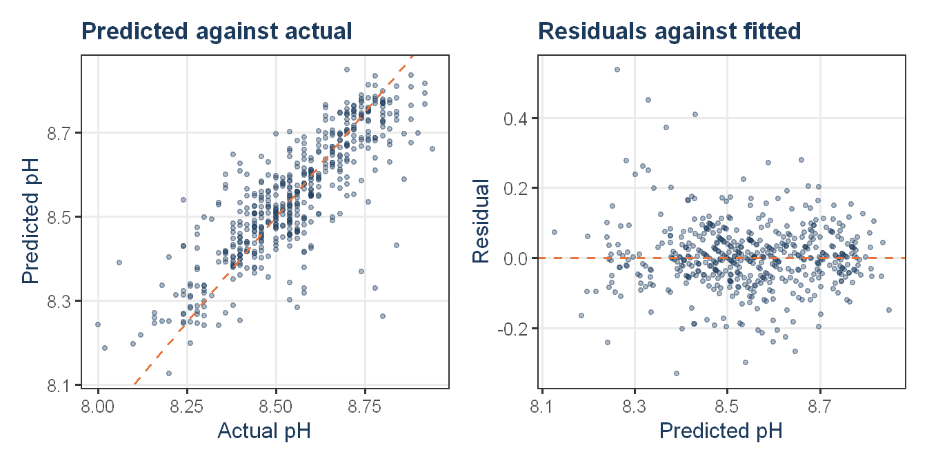
The residuals show the signature of a conditional-mean estimator, and it is the most important diagnostic in this appendix.

The point cloud rotates away from the diagonal at both ends. Runs with a true pH near 8.0 are predicted around 8.25, and runs near 8.9 are predicted closer to 8.8. The model systematically pulls its predictions toward the middle of the distribution, and the residual panel shows the same thing as a rising trend from left to right. This is not a defect to be tuned away. Any model that minimizes squared or absolute error will hedge toward the conditional mean where the predictors are ambiguous, and the extremes are exactly where they are most ambiguous.

The operational consequence is serious enough to justify the guardrail in the main report. The runs the model is worst at are the runs that fall outside specification, which are the only runs anyone cares about catching. A batch heading for 8.0 will be predicted at 8.25 and may not trip an alarm. The model is a useful early warning for drift within the normal operating envelope and it is not a substitute for laboratory confirmation at the edges.

The horizontal banding in the left panel is the 0.02 measurement grid, not a modeling artifact. The actual values can only take 52 distinct levels, so they stack into rows.

Scoring the evaluation set

The champion is refit on all 2,567 usable runs at the tuning parameters cross-validation selected. The holdout has served its purpose and is folded back in, because discarding a fifth of the available data at the point of scoring would cost accuracy for no remaining benefit.

The accuracy figure quoted in the management report comes from the held-out model rather than this one. The shipped model is trained on twenty percent more data, so the quoted figure is if anything slightly conservative.

The 267 evaluation runs pass through the identical encoding, alignment and imputation objects that were fit on training data. That is what guarantees consistency between what the model learned and what it is asked to score.

# Refit the champion on all usable rows at the winning tuning parameters, then
# score. The holdout has done its job and is folded back in.
set.seed(SEED)
champion_final <- train(X_all, y_all,
                        method     = champion_cv$method,
                        preProcess = PP,
                        metric     = "MAPE",
                        maximize   = FALSE,
                        tuneGrid   = champion_cv$bestTune,
                        trControl  = trainControl(method = "none"))

ph_pred <- as.numeric(predict(champion_final, newdata = X_scr))

# Fail loudly rather than ship a bad file.
stopifnot(length(ph_pred) == nrow(raw_score), !any(is.na(ph_pred)))

out    <- read_raw(PATH_SCORE)
out$PH <- round(ph_pred, 3)
write.xlsx(out, PATH_OUT)

cat(sprintf("Predicted pH  n: %d | mean: %.3f | sd: %.3f | range: %.2f to %.2f\n",
            length(ph_pred), mean(ph_pred), sd(ph_pred),
            min(ph_pred), max(ph_pred)))

Predicted pH  n: 267 | mean: 8.555 | sd: 0.150 | range: 8.09 to 9.10

cat(sprintf("Historical pH n: %d | mean: %.3f | sd: %.3f | range: %.2f to %.2f\n",
            length(y_all), mean(y_all), sd(y_all), min(y_all), max(y_all)))

Historical pH n: 2567 | mean: 8.546 | sd: 0.173 | range: 7.88 to 9.36

cat("Wrote", PATH_OUT, "with", nrow(out), "predictions and",
    sum(is.na(out$PH)), "missing values.\n")

Wrote ../resources/PH_Predictions_Group3.xlsx with 267 predictions and 0 missing values.

bind_rows(
  tibble(PH = y_all,    Source = "Historical runs"),
  tibble(PH = ph_pred,  Source = "Predicted, evaluation runs")
) |>
  ggplot(aes(x = PH, fill = Source)) +
  geom_density(alpha = 0.55, color = NA) +
  scale_fill_manual(values = c("Historical runs" = proj_grey,
                               "Predicted, evaluation runs" = proj_navy)) +
  labs(title = "Predictions sit inside the historical range, and are narrower",
       subtitle = "A conditional-mean model does not reproduce the full spread of the response",
       x = "pH", y = "Density") +
  theme_proj()

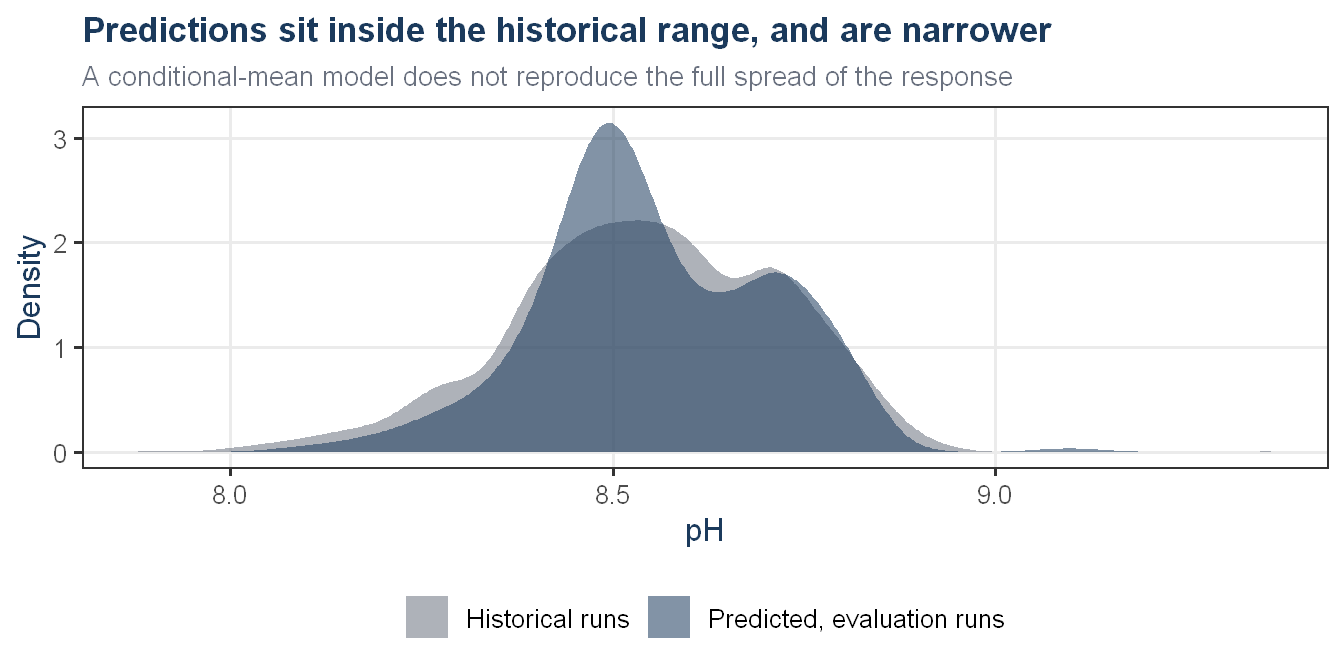
Appendix Figure A9. Predicted pH against the historical distribution

The predicted values have a standard deviation of 0.150 against 0.173 for the historical record, and they span 8.09 to 9.10 against a historical range of 7.88 to 9.36.

Both facts are expected and neither is a defect. A regression model predicts a conditional mean, so its output carries only the variation the predictors can explain and none of the residual variation. With an R-squared of 0.69, the predictions should carry roughly the square root of that share of the response’s spread, which is 0.143 against the 0.150 we observe. A prediction set that reproduced the full historical spread would be evidence of a model fitting noise, not of a model being accurate.

The narrower range is the same phenomenon seen from the other side. It is worth being precise about the mechanism, because the loose claim that a model like this cannot produce a value outside its training range is not true of Cubist. Each rule terminates in a local linear model, and a linear model is unbounded. What holds the predictions in is the instance-based correction, which adjusts every rule output using the 5 nearest historical runs and therefore anchors it to responses that were actually observed, together with the shrinkage toward the conditional mean documented in the diagnostics above. The practical result is what we see here: nothing below 8.09 and nothing above 9.10. A batch genuinely heading for 7.9 will not be predicted at 7.9, which is why the range check is a requirement rather than a suggestion.

Limitations

The validation is honest but finite. Imputation is fit inside every fold and the holdout was opened once, so the reported figures are not inflated by leakage. They are still estimates from 2,567 runs of one plant over one period, and the confidence interval around a MAPE of 0.77 percent on 512 holdout runs is not negligible.

Importance is a property of the model, not of the plant. We demonstrated this directly: two models that predict pH about equally well disagree about whether chemistry or machine state matters more. We report both rather than choosing, but a reader should understand that no single importance ranking of this dataset is the truth, including ours.

Within the chemistry cluster no attribution is possible. The four measurements correlate above 0.90, they are not discardable, and the model assigns them coefficients that only make sense in combination. Any statement of the form “increasing X raises pH” for a chemistry variable is unsupported by this analysis and would be unsupported by any analysis of this data.

The model extrapolates unreliably, and it fails silently when asked to. Presented with conditions unlike anything in the historical record it returns a plausible number near the edge of its experience, with no signal that it is guessing. This is the failure mode most likely to cause harm, because it coincides exactly with the batches that are out of specification.

The response carries a measurement floor of 0.02 pH. A portion of what we report as model error is the resolution of the instrument we are being scored against, and no model can be tuned below it.

Finally, the model has a shelf life. It describes the plant as it ran in the historical record, and equipment, formulations, sensors and recipes all change. Accuracy should be re-measured against fresh laboratory results on a schedule, and the model retrained when it degrades. A model that is quietly wrong is worse than no model, because it is trusted.

Bonus: R versus Python

Objective

Leadership is considering standardizing on one analytics platform. The question is not which language is more popular. It is whether a team that builds this model in Python arrives at the same answer as a team that builds it in R, and where any difference actually comes from.

We rebuilt the pipeline in Python on the same data, the same dropped rows, the same brand encoding, the same missingness flag, the same near-zero-variance removal, the same 80/20 split indices and the same selection metric. Every difference that remains is therefore a property of the platform or of our own tuning choices, and not of a different analyst preparing the data differently.

# Python runs in this document. Results cross the bridge as a CSV round trip,
# and all plotting stays in R under the shared theme.
library(reticulate)

py_require(c("pandas", "numpy", "scikit-learn", "openpyxl"))

py_to_r_df <- function(obj) {
  if (inherits(obj, "data.frame")) obj
  else utils::read.csv(text = obj$to_csv(index = FALSE))
}

# Zero-based training indices, so Python trains on exactly the rows R did.
py_idx_train <- as.integer(idx_train) - 1L

The same pipeline in Python

The encoded matrices are handed to Python directly. Re-deriving the feature matrix in pandas would introduce differences in dummy coding and column order that have nothing to do with the modeling libraries, and would turn this into a test of two people’s data wrangling rather than of two platforms.

The one preprocessing detail that requires care is the imputation. caret’s knnImpute centers, scales, then imputes on the scaled data. The scikit-learn equivalent is a StandardScaler followed by a KNNImputer, both inside a Pipeline, so that GridSearchCV refits them on each fold’s training rows only. Fitting the imputer once on the full training set before cross-validating is the same leakage error described in the appendix.

import os
import warnings
import numpy as np
import pandas as pd
from sklearn.base import clone
from sklearn.pipeline import Pipeline
from sklearn.preprocessing import StandardScaler
from sklearn.impute import KNNImputer
from sklearn.model_selection import GridSearchCV, KFold
from sklearn.linear_model import LinearRegression, ElasticNet
from sklearn.cross_decomposition import PLSRegression
from sklearn.svm import SVR
from sklearn.ensemble import RandomForestRegressor, GradientBoostingRegressor

# StandardScaler emits these while doing NaN-aware reductions. Nothing is wrong.
warnings.filterwarnings("ignore", category=RuntimeWarning)

SEED = 624

X_all = pd.DataFrame(r.X_all)
y_all = np.asarray(r.y_all, dtype=float)
X_scr = pd.DataFrame(r.X_scr)[X_all.columns]

idx_train = np.asarray(r.py_idx_train, dtype=int)
idx_test  = np.setdiff1d(np.arange(len(y_all)), idx_train)

X_train, y_train = X_all.iloc[idx_train], y_all[idx_train]
X_test,  y_test  = X_all.iloc[idx_test],  y_all[idx_test]


def mape(obs, pred):
    return float(np.mean(np.abs((obs - pred) / obs)) * 100)


# Negated because GridSearchCV maximizes.
def mape_scorer(est, X, y):
    return -mape(y, est.predict(X))


# Scaler and imputer sit inside the pipeline, so GridSearchCV refits both on
# each fold's training rows only. This mirrors knnImpute inside caret's train().
def make_pipe(model):
    return Pipeline([
        ("scale",  StandardScaler()),
        ("impute", KNNImputer(n_neighbors=5)),
        ("model",  model),
    ])


# PLSRegression returns a column vector, which breaks the shared scorer.
class PLSFlat(PLSRegression):
    def predict(self, X, copy=True):
        return super().predict(X, copy=copy).ravel()


# n_jobs is 1 throughout. joblib cannot spawn worker processes from an
# interpreter embedded inside R, so any parallel backend fails immediately.
slate = {
    "Linear Regression": (LinearRegression(), {}),
    "PLS":               (PLSFlat(),
                          {"model__n_components": list(range(1, 16))}),
    "Elastic Net":       (ElasticNet(max_iter=10000, random_state=SEED),
                          {"model__alpha":    [0.001, 0.01, 0.1, 1.0],
                           "model__l1_ratio": [0.1, 0.5, 0.9, 1.0]}),
    "SVM (radial)":      (SVR(kernel="rbf"),
                          {"model__C":     [1, 4, 16, 64],
                           "model__gamma": ["scale", 0.01, 0.03]}),
    "Random Forest":     (RandomForestRegressor(n_estimators=500,
                                                random_state=SEED, n_jobs=1),
                          {"model__max_features": [8, 14, 20, 26]}),
    "GBM":               (GradientBoostingRegressor(learning_rate=0.05,
                                                    random_state=SEED),
                          {"model__n_estimators": [500, 1000],
                           "model__max_depth":    [3, 5, 7]}),
}

folds = KFold(n_splits=10, shuffle=True, random_state=SEED)

# The grid searches are slow and single-threaded, so results are cached to disk.
# Delete the two CSV files to refit from scratch.
CACHE_RESULTS = "../resources/py_results.csv"
CACHE_PREDS   = "../resources/py_preds.csv"

if os.path.exists(CACHE_RESULTS) and os.path.exists(CACHE_PREDS):
    py_results = pd.read_csv(CACHE_RESULTS)
    _preds     = pd.read_csv(CACHE_PREDS)
    py_pred    = _preds["py_pred"].to_numpy()
    py_pred_rf = _preds["py_pred_rf"].to_numpy()
    print("Read cached results. Delete", CACHE_RESULTS, "to refit.")
else:
    rows, fitted = [], {}
    for name, (model, grid) in slate.items():
        print("fitting", name, flush=True)
        search = GridSearchCV(make_pipe(model), grid, scoring=mape_scorer,
                              cv=folds, n_jobs=1, refit=True)
        search.fit(X_train, y_train)
        fitted[name] = search.best_estimator_
        rows.append({
            "Model":     name,
            "CV_MAPE":   -search.best_score_,
            "Test_MAPE": mape(y_test, search.predict(X_test)),
        })

    py_results = pd.DataFrame(rows).sort_values("CV_MAPE").reset_index(drop=True)

    # best_estimator_ is already a configured pipeline. Clone, refit on all
    # usable rows, and score the 267 evaluation runs.
    py_pred    = clone(fitted[py_results.loc[0, "Model"]]).fit(X_all, y_all).predict(X_scr)
    py_pred_rf = clone(fitted["Random Forest"]).fit(X_all, y_all).predict(X_scr)

    py_results.to_csv(CACHE_RESULTS, index=False)
    pd.DataFrame({"py_pred": py_pred,
                  "py_pred_rf": py_pred_rf}).to_csv(CACHE_PREDS, index=False)

Read cached results. Delete ../resources/py_results.csv to refit.

py_champion = py_results.loc[0, "Model"]

print(py_results.to_string(index=False))

            Model  CV_MAPE  Test_MAPE
              GBM 0.788804   0.759548
    Random Forest 0.822611   0.798907
     SVM (radial) 1.065724   1.015902
Linear Regression 1.232055   1.138662
      Elastic Net 1.233004   1.139498
              PLS 1.235394   1.141339

print("\nPython champion:", py_champion)

Python champion: GBM

Two model families in the R slate have no scikit-learn counterpart. MARS has no maintained implementation in the library, and Cubist has none at all. Six models cross over, and those six are what the comparison rests on.

Do the two platforms agree?

py_results  <- py_to_r_df(py$py_results)
py_champion <- py$py_champion
py_row      <- py_results |> filter(Model == py_champion)

# The R random forest, refit on all rows and scored, so the two platforms can be
# compared on the same model family rather than best against best.
set.seed(SEED)
rf_final <- train(X_all, y_all,
                  method     = "rf",
                  preProcess = PP,
                  metric     = "MAPE",
                  maximize   = FALSE,
                  tuneGrid   = fit_rf$bestTune,
                  ntree      = 500,
                  trControl  = trainControl(method = "none"))

rf_pred_r  <- as.numeric(predict(rf_final, newdata = X_scr))
rf_pred_py <- as.numeric(py$py_pred_rf)
py_pred    <- as.numeric(py$py_pred)

gap_cv <- function(m) {
  abs(res_summary$CV_MAPE[res_summary$Model == m] -
      py_results$CV_MAPE[py_results$Model == m])
}

rf_gap_cv   <- gap_cv("Random Forest")
gbm_gap_cv  <- gap_cv("GBM")
svm_gap_cv  <- gap_cv("SVM (radial)")

rf_gap_test <- abs(res_summary$Test_MAPE[res_summary$Model == "Random Forest"] -
                   py_results$Test_MAPE[py_results$Model == "Random Forest"])

Bonus Table B1. MAPE values for the same models on the same holdout, both platforms.

res_summary |>
  select(Model, R_CV = CV_MAPE, R_Test = Test_MAPE) |>
  left_join(py_results |> select(Model, Py_CV = CV_MAPE, Py_Test = Test_MAPE),
            by = "Model") |>
  arrange(R_Test) |>
  style_ft(digits = 3)

Model	R_CV	R_Test	Py_CV	Py_Test
Cubist	0.795	0.773
Random Forest	0.823	0.801	0.823	0.799
GBM	0.914	0.881	0.789	0.760
SVM (radial)	1.008	0.974	1.066	1.016
MARS	1.094	1.049
Linear Regression	1.228	1.138	1.232	1.139
Elastic Net	1.229	1.138	1.233	1.139
PLS	1.232	1.138	1.235	1.141

The two platforms closely agree to 0.0001 MAPE points on cross-validation and 0.0025 on the identical holdout. The linear models are similarly indistinguishable. Both platforms are calling the same algorithms on the same rows and getting very similar answers, which is what we expected and what settles the language question.

Two rows do not behave that way, and they move in opposite directions. Gradient boosting differs by 0.125 MAPE points on cross-validation, roughly 863 times the random forest discrepancy, and Python is ahead. The radial SVM differs by 0.058 points, and Python is behind. A platform that simply fit better models would not lose one of these and win the other.

What produces the pattern is tuning. R’s gbm takes interaction.depth as the number of splits per tree, while scikit-learn’s max_depth is tree depth, so the value 7 buys a tree with seven splits in R and up to 128 leaves in Python. The defaults differ too, since gbm subsamples half the rows at each iteration and scikit-learn does not. On the SVM the asymmetry runs the other way, because caret’s svmRadial estimates the kernel width analytically from the data before searching cost, while our Python grid offered three hand-chosen values of gamma and then selected the smallest cost we supplied, which is the signature of a grid centered in the wrong place. In both cases we ported a grid across by name and searched a different model space than we thought we were searching.

Python’s gradient boosting therefore finishes ahead of our champion, at 0.7595 against Cubist’s 0.7729 on the holdout. However, that comes with a considerable computational cost. That said, the selection stands since Cubist beat the properly-tuned random forest on both routes, but a like-for-like gbm re-tune is the obvious next step.

parity <- tibble(
  R_Cubist = ph_pred,
  R_RF     = rf_pred_r,
  Py_RF    = rf_pred_py,
  Py_Best  = py_pred
)

cor_rf_rf   <- cor(parity$R_RF,     parity$Py_RF)
cor_cub_py  <- cor(parity$R_Cubist, parity$Py_Best)
max_gap_rf  <- max(abs(parity$R_RF     - parity$Py_RF))
max_gap_cub <- max(abs(parity$R_Cubist - parity$Py_Best))

# The single run where the two champions disagree most.
worst <- parity |> slice_max(abs(R_Cubist - Py_Best), n = 1)

p_lang <- ggplot(parity, aes(x = R_RF, y = Py_RF)) +
  geom_abline(slope = 1, intercept = 0, color = proj_grey, linetype = "dashed") +
  geom_point(alpha = 0.5, size = 1.2, color = proj_teal) +
  labs(title = "Same model, two languages",
       subtitle = sprintf("Random forest in each, r = %.3f", cor_rf_rf),
       x = "R prediction", y = "Python prediction") +
  theme_proj()

p_fam <- ggplot(parity, aes(x = R_Cubist, y = Py_Best)) +
  geom_abline(slope = 1, intercept = 0, color = proj_grey, linetype = "dashed") +
  geom_point(alpha = 0.5, size = 1.2, color = proj_navy) +
  labs(title = sprintf("Cubist against Python's %s", py_champion),
       subtitle = sprintf("Each platform's champion, r = %.3f", cor_cub_py),
       x = "R prediction (Cubist)",
       y = sprintf("Python prediction (%s)", py_champion)) +
  theme_proj()

p_lang + p_fam

Bonus Figure B1. Agreement on the 267 evaluation runs, by language and by model choice

The two panels answer two different questions, and only one of them is about Python.

The left panel is the language question. The same random forest, fit in two languages on the same rows, agrees on the 267 evaluation runs at a correlation of 0.998. For practical purposes the two languages produce the same predictions.

The right panel is the model question. The two platforms’ champions correlate at 0.936, with a largest single disagreement of 0.49 pH. The disagreement is not evenly spread, and where it concentrates is the part worth reading. Across the bulk of the operating range the two models track each other closely.

That is the finding worth taking to leadership. The choice of language moved our predictions by 0.041 pH. The choice of model can move them by 0.49 pH, while we need to consider the cost of computation and overhead each model and its proper tuning dictate. Python’s champion model took significantly longer with increased tree depth.

Where the platforms genuinely differ

Hyperparameters do not port by name. This is the practical lesson of the whole exercise and it cost us the most. interaction.depth and max_depth sound like the same knob and are not, and svmRadial estimates a kernel width that scikit-learn expects you to supply. Any team migrating a model between platforms has to re-tune from scratch, and a grid translated literally will quietly evaluate a different model than the one it names.

Parallelism in a mixed workflow. scikit-learn’s n_jobs does not work when Python is driven from R. joblib cannot spawn worker processes from an interpreter embedded inside another program, and on Windows the failure surfaces as a TerminatedWorkerError that says nothing about the real cause. Every Python model in this document was fit on a single core as a result. This is a cost of the hybrid setup, which parallelizes normally when run on its own, but it is a real cost for any team that plans to combine Python and R in the same environment. It can be said, almost without a doubt, that issues would arise if you were to run your R code from Python environment.

Near-zero variance. No direct equivalent. VarianceThreshold applies a variance rule and caret’s nearZeroVar applies a frequency-ratio rule, which is what identified Hyd.Pressure1. The rule has to be written by hand in Python. The honest claim is that there is no direct equivalent, not that Python cannot do it.

Breadth of the model library. Cubist and MARS have no scikit-learn implementation. That did not decide the accuracy contest here, but it did mean a Python-only team would never have evaluated the model that won our R comparison, and would not have known it was missing. However, besides scikit-learn, there are other packages in Python for the missing models.

Diagnostics. resamples() gives fold-level paired comparisons directly, which is what let us establish that Cubist beat the runner-up in 9 of ten folds rather than merely on average. scikit-learn carries the same information in cv_results_ but it has to be assembled.

Bonus Table B2. Platform comparison, each row argued from evidence in this project

tibble(
  Dimension = c("Accuracy, like for like",
                "Portability of a tuning grid",
                "Breadth of model library",
                "Preprocessing correctness",
                "Paired model comparison",
                "Deployment path"),
  Winner = c("Tie",
             "Neither",
             "R",
             "Tie",
             "R",
             "Python"),
  Evidence = c(
    sprintf("Random forest agrees to %.4f MAPE on the identical holdout.", rf_gap_test),
    sprintf("The same nominal grids differ by %.3f CV MAPE on GBM and %.3f on the SVM, in opposite directions.", gbm_gap_cv, svm_gap_cv),
    "Cubist and MARS have no scikit-learn implementation, and Cubist won the R comparison.",
    "Both are one line. Every leakage bug in this group's submissions was in R, and the one Python submission got it right.",
    "resamples() pairs folds directly. cv_results_ carries the same data but must be assembled.",
    "A fitted Pipeline carries scaler, imputer and model as one serializable object. The R equivalent is a caret object plus the encoding and alignment functions defined in this document."
  )
) |>
  style_ft()

Dimension	Winner	Evidence
Accuracy, like for like	Tie	Random forest agrees to 0.0025 MAPE on the identical holdout.
Portability of a tuning grid	Neither	The same nominal grids differ by 0.125 CV MAPE on GBM and 0.058 on the SVM, in opposite directions.
Breadth of model library	R	Cubist and MARS have no scikit-learn implementation, and Cubist won the R comparison.
Preprocessing correctness	Tie	Both are one line. Every leakage bug in this group's submissions was in R, and the one Python submission got it right.
Paired model comparison	R	resamples() pairs folds directly. cv_results_ carries the same data but must be assembled.
Deployment path	Python	A fitted Pipeline carries scaler, imputer and model as one serializable object. The R equivalent is a caret object plus the encoding and alignment functions defined in this document.

Recommendation

Do not standardize on a language. Standardize on the slate and the selection rule.

The evidence in this project does not support an accuracy case for either platform. Where we compared like for like, the two agreed on the identical holdout. Where they disagreed, they disagreed in both directions, and the cause in each case was a tuning grid that did not survive translation rather than a difference in what the libraries can fit. Both platforms reached the high seven-tenths of a percent with a well-tuned tree ensemble.

So the requirement to impose is a floor, not a language. Any team modeling pH on this line should fit at least one linear baseline, one non-linear model and two or more tree and rule-based models, tune and select on the metric the business is scored on, and confirm on a holdout opened once. A team meeting that floor, will land close to the answer regardless of the language it uses. A team that does not, will ship a defensible-looking model that is worse than one it never tried.

If a single platform must be named for operational reasons, name R for the R&D and Python for the deployment. R’s slate is broader without additional dependencies, its resampling diagnostics are more direct, and it does not lose its cores to an embedding problem on the machines this team actually uses. Python’s fitted pipelines are a single serializable object and are closer to a service that can run against live sensor readings on the plant floor. However, neither of those is the reason this project produced a good model; the slate was.